
Hi everyone!
Over the last few days I have been working on a new Spring Boot starter for Oracle Spatial. I did this work with two other real developers, and three AI coding assistants, and I thought it would be interesting to write up the story of how it came together.
This was a good example of how building a starter is not just about getting code to compile or getting a sample app to run. It is also about API shape, developer expectations, reviewer feedback, naming, documentation, tests, and all of those little choices that decide whether something feels natural or awkward once another developer actually tries to use it.
We ended up in a much better place than where we started, but not because the first design was perfect. We got there because the reviews were good, the feedback was honest, and we were willing to change direction once it was clear the API could be better.
So this post is a bit of a behind-the-scenes look at that process.
What we were trying to build
The goal sounded simple enough on paper:
- create a Spring Boot starter for Oracle Spatial
- make it easy to work with
SDO_GEOMETRY - keep the programming model GeoJSON-first
- provide a sample application that shows realistic use
The kinds of queries we had in mind were the kinds of queries almost everyone reaches for first:
- store a point or polygon
- fetch it back as GeoJSON
- find landmarks near a point
- find landmarks within or interacting with a polygon
So from the beginning this was going to involve Oracle Spatial operators such as:
SDO_UTIL.FROM_GEOJSONSDO_UTIL.TO_GEOJSONSDO_FILTERSDO_RELATESDO_WITHIN_DISTANCESDO_NNSDO_GEOM.SDO_DISTANCE
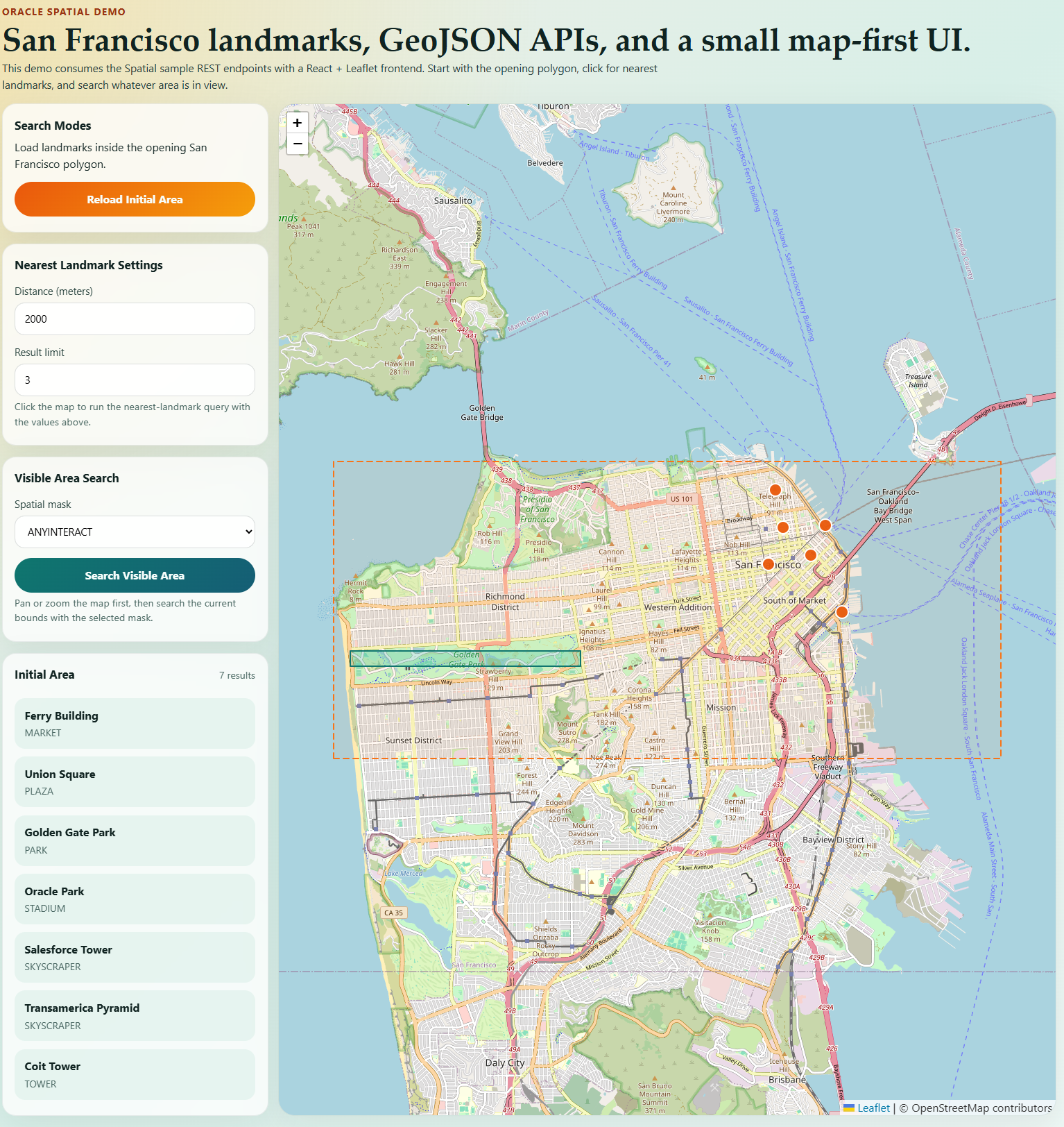
We also wanted a sample app that felt approachable. We used a small San Francisco landmark dataset so the sample would be easy to understand and a little bit fun to play with.
Where we started
The first version of the starter leaned in the direction that I think a lot of us would naturally start with: helper utilities.
We had one piece focused on converting GeoJSON to and from Oracle Spatial, and another piece focused on generating the bits of SQL you need for common spatial predicates and projections.
On one level, that worked.
It absolutely solved real problems:
- you did not have to remember the exact
SDO_UTIL.FROM_GEOJSON(...)call - you did not have to hand-type the common predicate shapes every time
- you could centralize the default SRID and distance unit
If you already like building SQL with JdbcClient, it was useful.
But there was a catch. The public API was still basically returning strings. And once that got called out in review, it was hard to ignore.
The review comment that changed everything
The most important reviewer comment was not about a syntax error or a missing test. It was about the shape of the API.
The feedback was basically: if this is a Spring Boot starter, why is the main experience a SQL string builder?
That was the right question.
It is one thing to have Spring-managed beans. It is another thing entirely to have a Spring-native programming model.
At that point the starter was Spring-managed, but not really Spring-native. Yes, you could inject the beans, but what you got back were still string fragments that you had to splice together yourself.
That triggered the main redesign.
The moment that made the redesign easier
One thing that helped a lot is that the original API had not been released yet.
That is a huge advantage.
It meant we did not need to protect old method names or preserve an API shape just because it already existed. We were free to ask a better question: if we were designing this from scratch for Spring developers, what should it look like?
Once we reframed it that way, the answer became much clearer.
What we changed
The big change was moving away from public string-builder beans and toward one main Spring JDBC integration bean:
OracleSpatialJdbcOperations
Instead of treating Oracle Spatial as a collection of string helper methods, we moved to a design where application code injects one bean and then creates typed spatial query parts:
SpatialGeometrySpatialExpressionSpatialPredicateSpatialRelationMask
This ended up being a much better fit for the way Spring JDBC code is usually written.
You still write SQL. We did not try to invent a whole DSL. But the spatial pieces now carry more meaning and stay connected to the bind process instead of floating around as anonymous fragments.
That was the key design improvement.
Why this felt better almost immediately
One of the things I liked about the redesign is that the sample application got better almost immediately once the API got better.
That is usually a good sign.
When an API is awkward, the sample tends to look awkward too. You can hide that for a little while, but not for long.
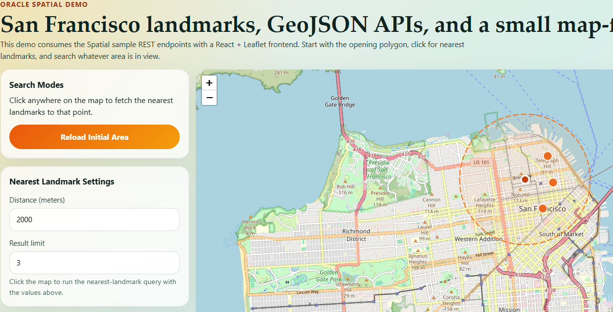
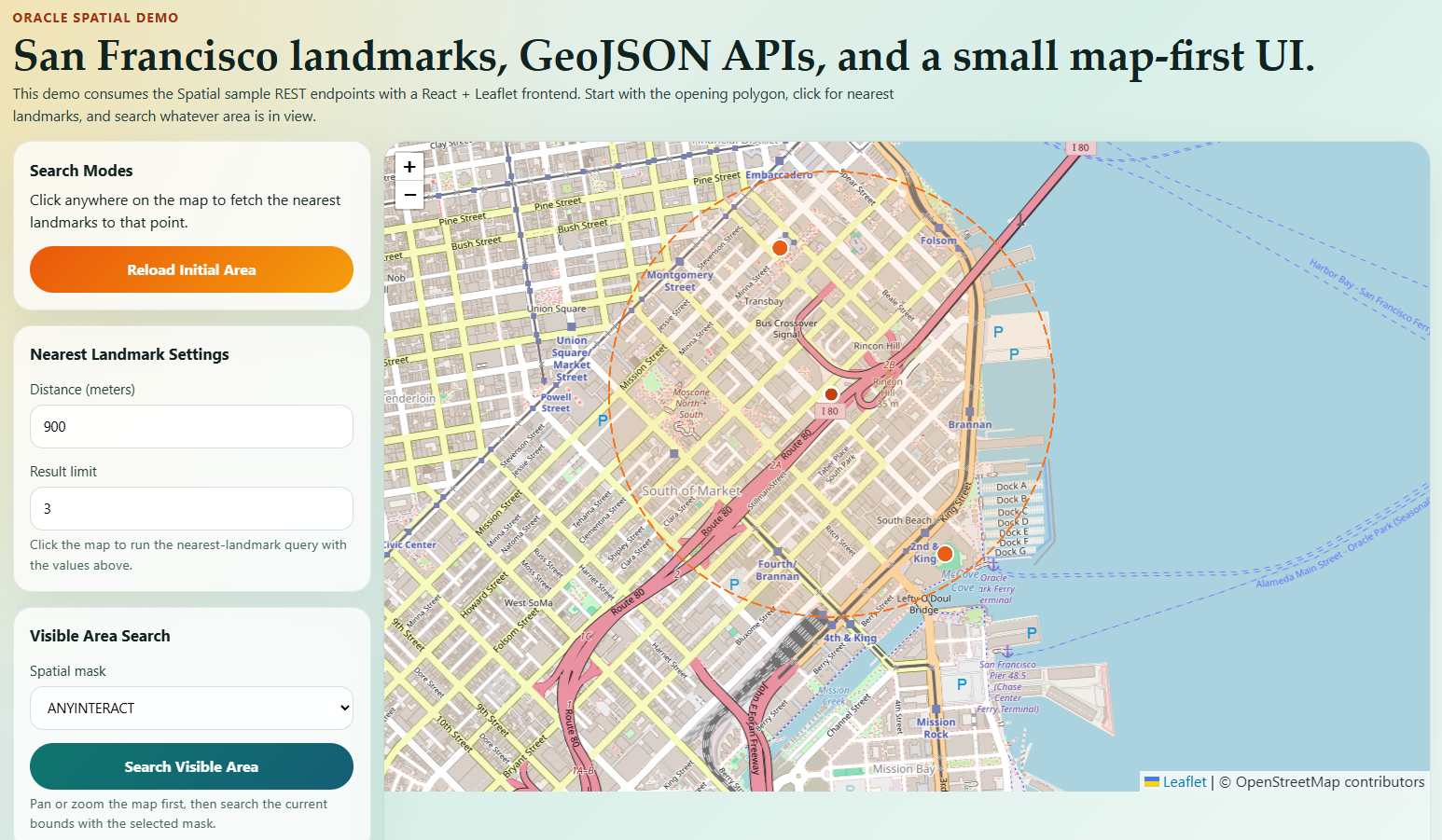
With the redesigned API, the service code started to read much more naturally. In the sample’s findNear flow, for example, we now create:
- a
SpatialGeometry - a distance expression
- a within-distance predicate
and then build the SQL around those named pieces.
That may sound like a small thing, but it makes a big difference when someone is reading the sample for the first time and trying to understand the intended usage pattern.
Instead of “here is some mysterious Oracle SQL,” the code reads more like “here is the geometry we are searching around, here is the distance we want to project, and here is the predicate we want to apply.”
That is a much better teaching story.
The sample app became part of the design process
I think sometimes people talk about sample applications as though they are just an afterthought. In practice, for a starter like this, the sample is part of the design process.
It answers questions like:
- does the API feel natural in a real service?
- are the method names understandable?
- can we explain this to somebody without too much ceremony?
- does the code read like Spring, or does it read like a thin wrapper over raw SQL?
Our sample app is a simple REST service built around landmarks in San Francisco.
It has endpoints for:
- creating a landmark
- fetching a landmark by id
- finding nearby landmarks
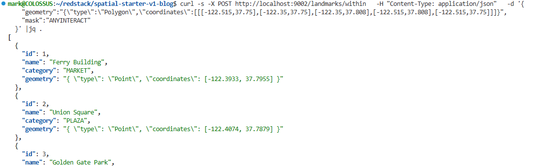
- finding landmarks inside or interacting with a polygon
We also spent some time improving the seed data because I wanted the sample to be a little more recognizable and useful. So the sample now includes landmarks like:
- Ferry Building
- Union Square
- Golden Gate Park
- Oracle Park
- Salesforce Tower
- Transamerica Pyramid
- Coit Tower
That may not be the most “architectural” part of the work, but it helps make the sample feel real instead of abstract.
One small enum that mattered more than I expected
Another design decision that turned out to matter a lot was replacing raw relation-mask strings with an enum:
SpatialRelationMask
This came directly out of review feedback.
The problem with raw strings is obvious once someone points it out: a developer can type something like "INTERSECTS" and everything looks fine until runtime, when Oracle tells them that is not a valid mask.
That is exactly the kind of thing a good starter should help with.
By introducing an enum, we made that part of the API:
- safer
- easier to discover
- harder to misuse
It is a small API element, but it made the whole thing feel more deliberate.
Distance became first-class because it had to
One of the early reviews also pointed out that if we wanted to serve real spatial use cases, we needed first-class support for distance calculations.
That was absolutely right.
A lot of real applications want some version of:
- find nearby things
- return the distance
- order by distance
If the starter handled filtering but not distance calculation, it would always feel like it stopped just short of the most useful scenario.
So SDO_GEOM.SDO_DISTANCE became part of the main API design rather than something developers would have to improvise themselves.
I think that made the starter much more credible for real use.
Documentation ended up being more important than I expected
I do not mean that in a generic “docs matter” way. I mean that for this starter in particular, the documentation had to explain a mental model, not just list methods.
The most useful documentation change we made was adding a clear distinction between:
- what gets injected as a Spring bean
- what gets created per query
That turned out to be the right way to explain the design.
You inject:
OracleSpatialJdbcOperations
And then per query you create:
SpatialGeometrySpatialExpressionSpatialPredicate
Once we started explaining it that way, the docs got much easier to follow.
We also added concrete query pattern examples for:
- inserts
- GeoJSON projection
- filter + relate
- distance-ordered proximity queries
Those examples matter because they show how the design is actually supposed to be used. For a starter, that is every bit as important as the Javadoc.
Some of the polish came from the less glamorous review comments
Not all of the useful review feedback was high-level architecture. Some of it was the kind of practical feedback that makes software much more solid.
A few examples:
The sample needed better error handling
At one point the sample app would throw an exception and return a 500 if a caller passed an invalid spatial relation mask.
That is a perfectly believable bug in a sample. It is also exactly the kind of thing a reviewer should call out, because the sample is part of the product story.
We fixed it so that invalid masks now produce a proper 400 Bad Request with a useful message.
The tests needed to be more Spring-native too
We got feedback to use @ServiceConnection in the Testcontainers-based tests, and that was good advice. It made the tests more consistent with current Spring Boot style and reduced some manual wiring.
We also adjusted the integration test to run as the app user rather than system, which is a much better representation of how the code should actually work.
The SQL setup needed to be repeatable in CI
This is one of those things that only becomes obvious once CI starts yelling at you.
We hit issues with setup SQL being run more than once and colliding with existing objects or metadata. That led to a round of cleanup to make the test setup more idempotent and more robust.
That is not the glamorous part of building a starter, but it is absolutely part of shipping one.
What we deliberately did not do
There were also some things we chose not to do in this round of work.
I think that is worth talking about because saying “not yet” is often part of good design.
We did not try to eliminate SQL entirely
Even after the redesign, application code still assembles SQL statements with JdbcClient.
That was intentional.
We wanted to make the API more Spring-native, but not disappear into a custom DSL or pretend SQL no longer exists. This is still Spring JDBC. SQL is still the right abstraction level. The important improvement was to stop making the public API itself a string-builder API.
There is still room to improve the ergonomics in the future, especially around making it harder to forget a bind contributor. Reviewers called that out too, and I think they are right. But that felt like a v2 refinement, not something we needed to solve before this version was useful.
We did not add every possible spatial operation
Another good review point was that buffer generation would be useful too. I agree.
But once again, that felt like feature expansion rather than a cleanup item for this iteration.
There is always a temptation to keep adding one more thing once the codebase is open and fresh in your mind. In this case I think the right move was to get the core API shape right, get the sample and docs into good condition, and leave some room for future work.
What I think we ended up with
At the end of all of this, what we have is not just a set of helper methods. It is a small but coherent Spring Boot story for Oracle Spatial.
The final result includes:
- a starter that auto-configures a Spring JDBC-oriented spatial bean
- a typed API for spatial query parts
- safer handling of
SDO_RELATEmasks - first-class distance support
- a sample REST app that demonstrates realistic usage
- docs that explain the mental model, not just the method list
- integration tests that run against Oracle AI Database 26ai Free with Testcontainers
And maybe the biggest thing for me is that it now feels like something I would want another Spring developer to pick up and try.
That was not as true of the first version.
What we are already thinking about for v2
Even though I feel good about where this landed, we have also been pretty careful to write down the things that did not belong in this iteration.
There are at least two clear areas for a possible v2.
The first is improving the ergonomics around binding and query composition.
Right now the design is much better than the original string-builder approach, but there is still a pattern like this:
spatial.bind( jdbcClient.sql("select ... " + distance.selection("distance") + " from landmarks where " + within.clause()), distance, within)
That is a reasonable place to be for a JDBC-oriented starter, but it is not hard to imagine a future version that tightens that up further and makes it harder to forget a bind contributor.
The second is expanding the supported spatial operations.
One of the most obvious candidates there is buffer generation with SDO_GEOM.SDO_BUFFER. That came up during review, and I think it is a very good candidate for a future enhancement. There are also broader questions about whether repository-style integrations or richer mapping options might make sense once we have real experience with how people use the current API.
But I want to be careful here. Just because we can imagine a v2 does not mean we should rush into it. What I would really like at this point is to get feedback from actual users first.
I would much rather learn from people who try the starter on real spatial workloads than guess too aggressively about what the next abstraction should be. Maybe the next thing we need is buffer support. Maybe it is better row mapping. Maybe it is a tighter JdbcClient integration. Maybe it is something we have not even thought about yet.
So yes, we do have a v2 plan taking shape. But before we take that next step, I would love to hear from users and see how this first version holds up in practice.
Working with AI coding assistants
Like many people today, I am doing more and more work with AI Coding assistants. For this piece of work, these are the participants and the roles they played:
- me: collaborated with GPT to write the specification, set the standards, conventions, etc., guided the whole process, read and reviewed code myself, helped make, or made design decisions
- GPT-5.4: acted as the primary developer, wrote most of the code, reflected on its own work, helped write and refine the specification, processed review comments and planned, helped with the design
- Claude Code: acted as a “senior architect” who reviewed the code with a focus on technical aspects and gave detailed feedback and recommendations
- Gemini (3 thinking/pro): acted as the “product manager” who reviewed the project from the point of view of how well it addressed the need, if it exposed the right features and capabilities, and how useful it would be for a spatial user
- two human colleagues: acted as reviewers and developers who provided valuable feedback on the code and the design
As we worked through the project together, I saved a lot of the generated plans and reviews in the .ai directory because I think those are valuable artifacts. We’re obviously using AI more, and we have no intention of hiding it, so why not save these for future use? Seems like the right thing to do. We did have a conversation about this before coming to the conclusion that we should save them and put them in the public repo.
I also want to mention that there were several cycles in the project. We started discussing the requirements and writing a plan. We reviewed this and iterated on it two or three times before we ever started writing any code. By “we”, I mean me and the three AIs. It was interesting to see the slightly different opinions of the AIs and the different areas they focused their attention on. Just like human developers, the different opinions and insights were useful to help us get to a better result.
After we started development, we continued to cycle through reviews, feedback, updates. At one point, as discussed above, we decided to redesign – this was a result of human feedback. The AIs certainly did a good job, and they are getting better all the time, but I do still feel that they are not as good at doing novel things as they are at doing things that have been done before, and they perhaps don’t consider (or at least mention) the implications of architectural decisions as much as some human developers do, at least in my experience to date. But I am sure they will continue to evolve rapidly.
I guess I’d just say – if you have not tried working in a team with multiple AI coding assistants yet, give it a go!
Why I wanted to write this up
I wanted to tell this story because I think it is a pretty normal and healthy example of how good API work actually happens.
You start with an idea.
You build something that is useful but not yet quite right.
Somebody asks a question that exposes the weakness in the design.
You resist it for a minute.
Then you realize they are right.
Then the real design work starts.
That is basically what happened here.
And I think the result is better precisely because we were willing to let the reviews change the direction of the code rather than just polish the original design.
Wrapping up
I am really happy with how this turned out.
Not because it is finished forever. It is not. There are still good future directions here. But the core design now feels solid, and the sample, tests, and docs all tell a coherent story.
That is what I wanted from this starter.
If you are working with Spring Boot and Oracle Database, and you have spatial use cases in mind, I think this gives you a pretty nice starting point. And if you are designing your own starter or library, maybe the bigger lesson here is that reviewer feedback is not just something to “address.” Sometimes it is the thing that helps you find the real design.


You must be logged in to post a comment.