
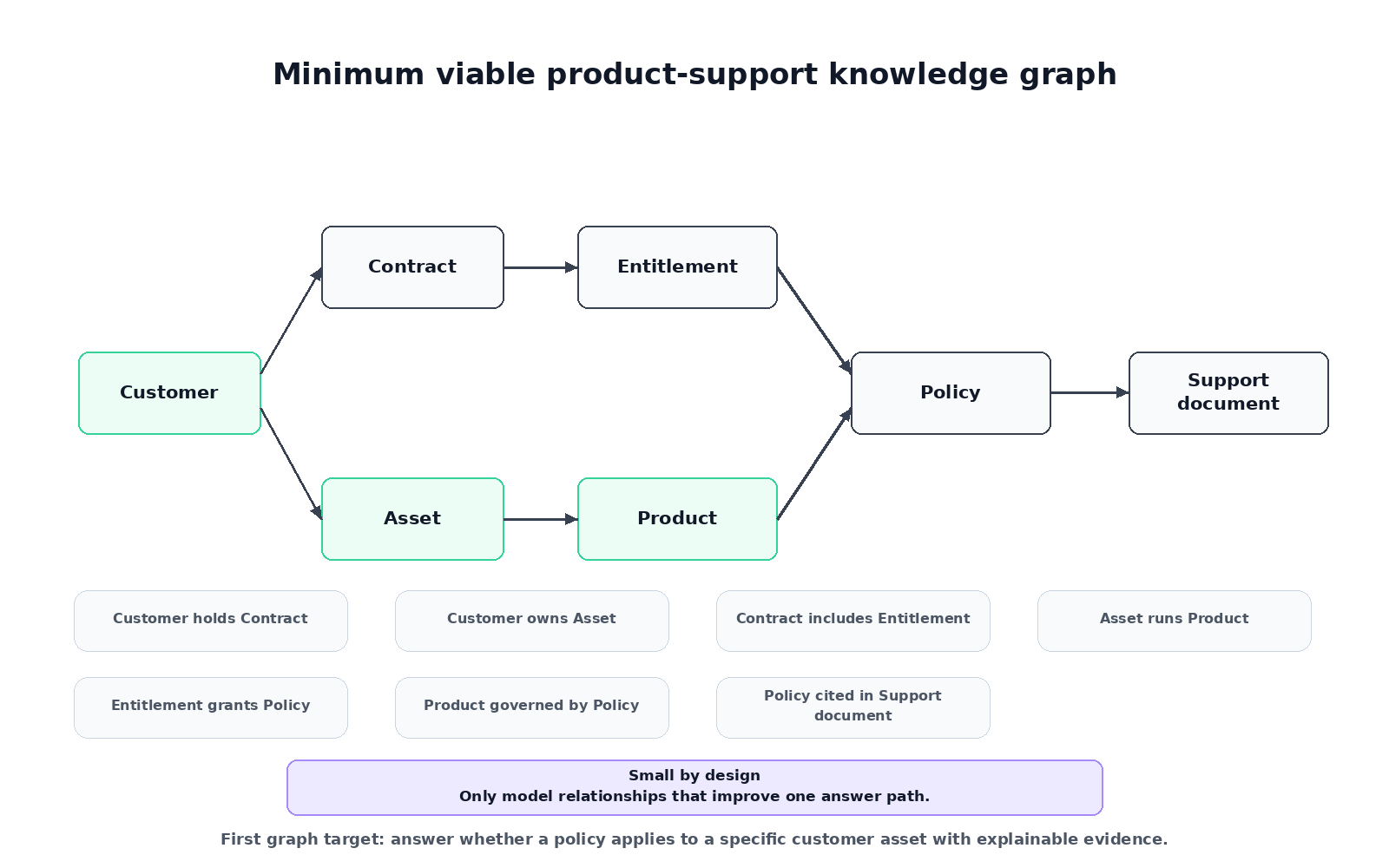
Grounded AI applications are hard to trust when the evidence is split across similar text, structured rows, and relationships. Flight disruption questions are a good example: a delayed traveler needs timing math, airport relationships, route alternatives, policy language, and a plain explanation that shows how the answer was reached. A basic RAG application can retrieve policy text, but it does not naturally understand that an inbound flight, a connection airport, an outbound segment, and an alternate route form a connected problem.
This tutorial builds a compact travel disruption assistant with Oracle AI Database 26ai, SQL property graphs, Oracle AI Vector Search, Python, and OpenAI. We will load staged tutorial CSVs shaped after OurAirports and BTS on-time performance fields, build a relational schema, define a SQL property graph, compare three retrieval modes, and generate a grounded answer to a missed-connection question.
The completed demo is intentionally small enough to inspect. It is not an operational airline recommendation system, and the included risk score is a deterministic tutorial ranking feature rather than a predictive model. The point is to show how graph-aware retrieval changes the evidence we can give an assistant.
What Is GraphRAG With Oracle AI Database 26ai?
GraphRAG combines graph traversal with retrieval-augmented generation. Instead of retrieving only text chunks that look semantically similar to the question, the application also follows relationships between entities: airports, flights, itinerary segments, connection rules, and candidate routes.
Oracle AI Database 26ai is a useful place to build this pattern because the same database can hold relational tables, vectors, and SQL property graph definitions. In this tutorial, policy chunks use vector retrieval, route facts stay in relational tables, and connected travel reasoning uses graph queries over the same stored data.
The demo calls OpenAI directly for embeddings and answer generation. The tutorial code keeps the OpenAI calls isolated in openai_provider.py, so the retrieval logic, schema, and graph queries remain clear.
Embeddings convert policy text and the user’s question into vectors so the database can compare meaning rather than only keywords. The stored policy vectors and the query vector must come from the same embedding model, because dimensions and numeric behavior are model-specific. If the OpenAI embedding model or configured embedding dimension changes, rebuild the stored policy vectors before comparing new queries with old rows.
Key Features of Oracle AI Database 26ai for GraphRAG
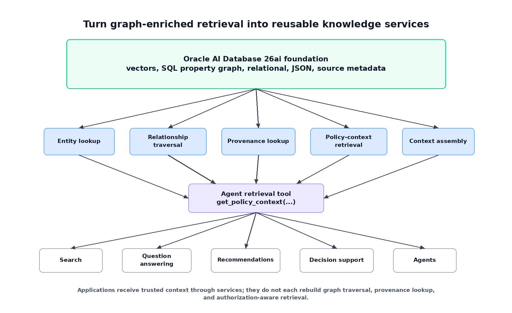
Oracle AI Database lets us keep structured, vector, and graph evidence close to the data. The demo uses a few features together rather than treating them as separate systems.
SQL property graphs
A SQL property graph exposes selected relational tables as vertices and edges. We model airports, passenger itineraries, and itinerary segments as vertices, then use route summaries, flight instances, and helper edge tables as relationships.
Oracle AI Vector Search
Policy chunks are stored with a VECTOR column and searched with VECTOR_DISTANCE(). The tutorial dataset has only a few policy chunks, so we keep the vector path simple and do not create an index in the runnable lab.
Relational constraints
Connection buffers, scheduled times, route risk scores, and passenger preferences are easier to inspect as relational rows. We use SQL for the pieces that should stay deterministic and explainable.
LLM-grounded answers
The final response is generated from retrieved evidence rather than from a free-form prompt. The OpenAI provider wrapper receives the question, evidence blocks, and explanation path, then returns an answer that the demo can inspect.
How to Get Started with Oracle AI Database 26ai GraphRAG
We will use the companion demo package generated with this tutorial. The public article shows the commands and representative snippets; the complete runnable files are in demo/demo_code_package.md and in the extracted demo workspace that accompanies this tutorial package.
Prerequisites:
- Python 3.12.
- Docker or a compatible Compose runtime for the included Oracle AI Database 26ai Free container.
- Access to Oracle Container Registry with the
database/freerepository terms accepted. - An OpenAI API key, an OpenAI generation model, an OpenAI embedding model, and the embedding dimension used for the vector column.
- The staged tutorial CSV files included in
data/raw.
The companion demo provisions Oracle AI Database 26ai Free locally with compose.yaml. The container startup mounts sql/10-setup-user.sql, creates a least-privilege graphrag_demo user in FREEPDB1, and leaves the Python checkpoint scripts to create only application-owned tutorial objects. You still supply your own OpenAI key and model identifiers, but you do not need a pre-created Oracle schema. The Python examples use python-oracledb thin mode by default; thick mode is useful when an environment requires Oracle Client libraries or wallet-specific client features.
Create the environment from the extracted demo project root:
docker compose up -dcp .env.example .envpython3 -m venv .venvsource .venv/bin/activatepython -m pip install --upgrade pippython -m pip install -r requirements.txt
Edit .env and replace only the OpenAI placeholders. The Oracle values already match the local Compose database and demo user created by the init SQL script. Do not commit .env, credentials, private endpoints, wallet files, or API keys:
ORACLE_USER=graphrag_demoORACLE_PASSWORD=GraphRAG_26ai_Demo1ORACLE_DSN=localhost:1521/FREEPDB1OPENAI_API_KEY=replace-with-openai-api-keyOPENAI_MODEL=replace-with-openai-generation-modelOPENAI_EMBEDDING_MODEL=replace-with-openai-embedding-modelOPENAI_EMBEDDING_DIMENSION=replace-with-embedding-model-dimension
Before you run the checkpoint scripts, look at the shared helper file. Most of the demo imports demo_common.py, so understanding it makes the rest of the workflow feel like a system instead of a series of magic commands.
dataclass(frozen=True)class Settings: oracle_user: str oracle_password: str oracle_dsn: str openai_api_key: str openai_model: str openai_embedding_model: str vector_dimension: int
The Settings object separates database connectivity, OpenAI generation, and OpenAI embeddings. That separation matters because each part changes at a different pace. If the embedding dimension changes, the vector table must be rebuilt. If the generation model changes, the schema and graph queries can stay the same.
The environment loader also validates a bug-prone value early:
def load_settings() -> Settings: # Keep the vector table shape aligned with the embedding model. dimension_text = require_env("OPENAI_EMBEDDING_DIMENSION") try: dimension = int(dimension_text) except ValueError as exc: raise RuntimeError("OPENAI_EMBEDDING_DIMENSION must be an integer") from exc if dimension <= 0: raise RuntimeError("OPENAI_EMBEDDING_DIMENSION must be greater than zero")
This is more than defensive programming. Vector search depends on a fixed dimension. A query vector with one dimension count cannot be compared against stored vectors with another, so a typo in .env should stop the run before any database rows are loaded.
The CSV fixtures are small tutorial extracts. They follow the field shape needed for the lab, but they are not real-time operational flight feeds.
Before loading them, inspect the shape. The staged airport file is intentionally tiny:
| airport_code | airport_name | airport_type | municipality | region_code |
|---|---|---|---|---|
| JFK | John F Kennedy International | large_airport | New York | US-NY |
| ORD | Chicago O’Hare International | large_airport | Chicago | US-IL |
| SFO | San Francisco International | large_airport | San Francisco | US-CA |
| DEN | Denver International | large_airport | Denver | US-CO |
| DFW | Dallas Fort Worth International | large_airport | Dallas-Fort Worth | US-TX |
The staged flight file keeps the delay and distance columns that the route summary uses later:
| flight_date | carrier | flight_number | origin | dest | dep_delay | arr_delay | cancelled | distance |
|---|---|---|---|---|---|---|---|---|
| 2025-01-03 | OC | 410 | JFK | ORD | 45 | 23 | 0 | 740 |
| 2025-01-04 | OC | 410 | JFK | ORD | 15 | 18 | 0 | 740 |
| 2025-01-03 | OC | 821 | ORD | SFO | 10 | 14 | 0 | 1846 |
| 2025-01-04 | OC | 821 | ORD | SFO | 62 | 70 | 0 | 1846 |
| 2025-01-03 | OC | 603 | ORD | DEN | 8 | 11 | 0 | 888 |
GraphRAG Travel Disruption Assistant Demo Project
The demo answers this question:
My flight from JFK to ORD is delayed by 45 minutes. I have a connecting flight from ORD to SFO. Can I still make it, and what should I do?
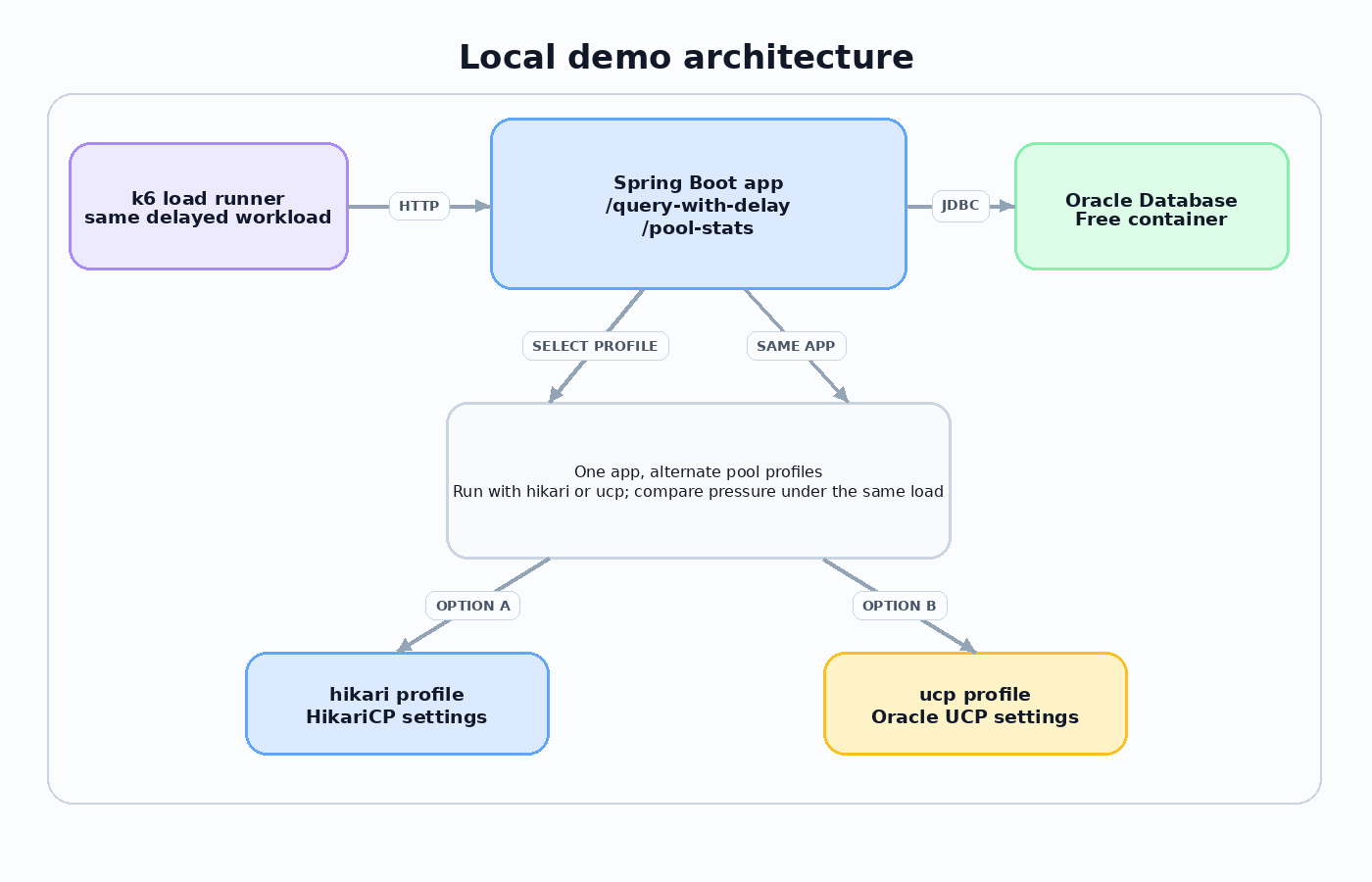
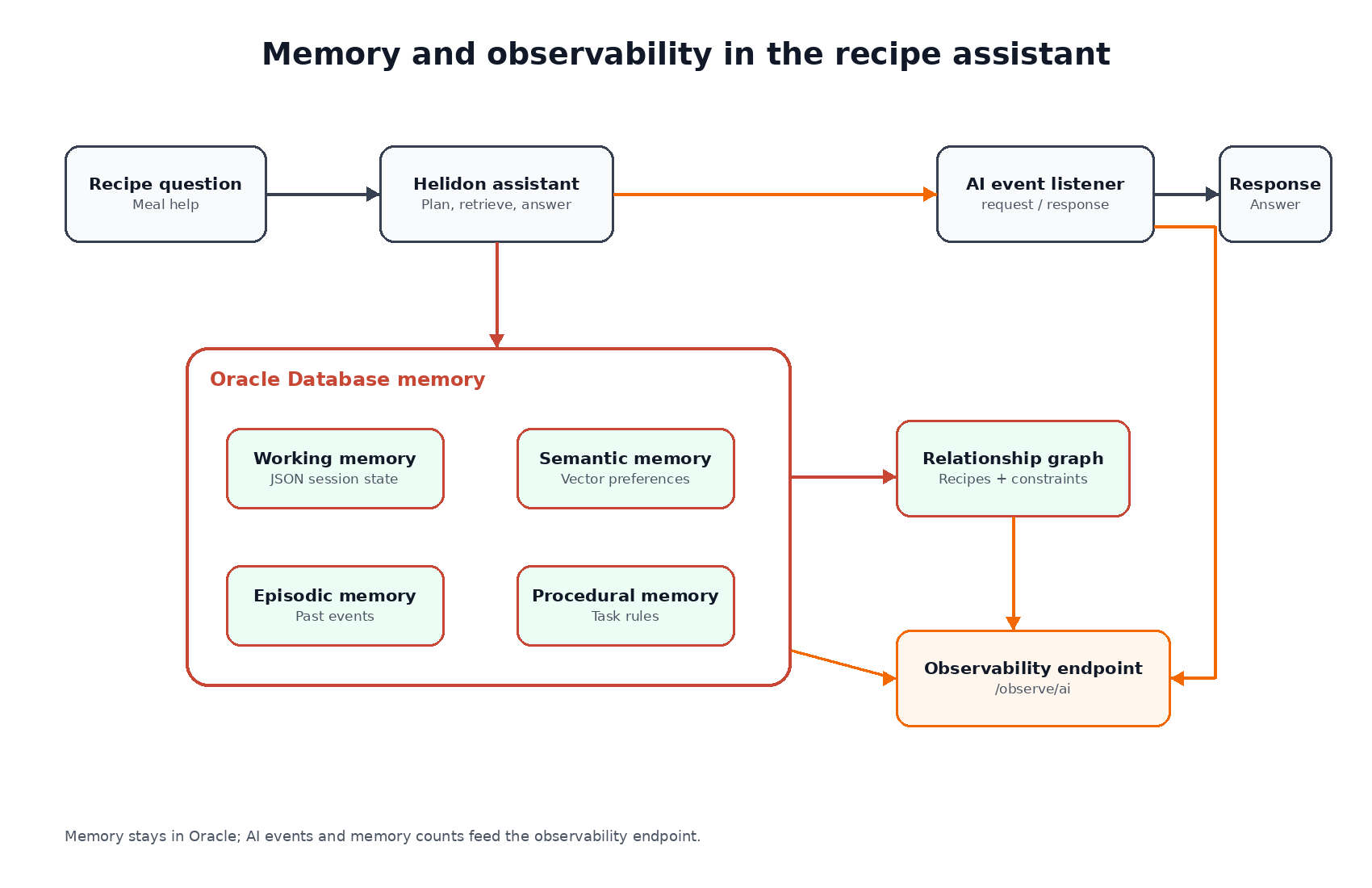
We will build three retrieval modes:
- Mode A: plain policy RAG.
- Mode B: policy RAG plus relational itinerary and route facts.
- Mode C: policy RAG plus relational facts plus SQL property graph traversal.
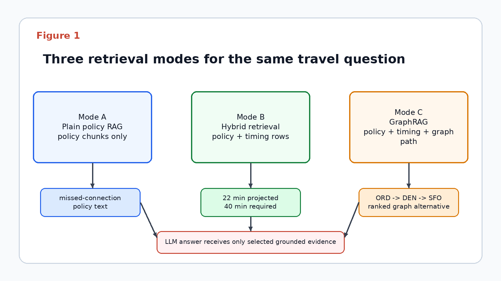
The retrieval-mode diagram shows why the rest of the demo is organized as a comparison. Each mode adds a kind of evidence: policy text, structured itinerary timing, and finally the graph path that exposes the DEN alternative.
The route graph is not abstract. It connects a delayed JFK to ORD segment, an at-risk ORD to SFO segment, and a ranked ORD to DEN to SFO alternative.
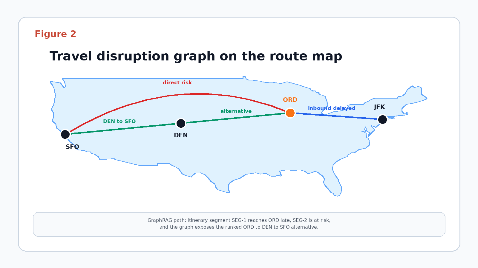
The map outline is derived from Natural Earth public-domain vector data, and the airport nodes use the latitude and longitude values from the staged airport fixture.
Basic
Step 1: Check the environment
First, run the environment check. It verifies required environment variables and database connectivity without printing secrets.
python 00_check_environment.py
Expected output:
Required database variables: presentOpenAI configuration: presentDatabase connection: OKDatabase identity: <Oracle AI Database banner>Environment check: OK
The check does not print secret values. It only confirms that the names needed by demo_common.py and openai_provider.py are present.
The check script is intentionally small. It calls the same settings loader used by later scripts and runs a banner query against the database. Treat it as a contract test for the workspace: if this step fails, fix the environment, dependency installation, or database connectivity before debugging graph SQL or answer generation.
Step 2: Create the schema
Next, create the database objects. The schema includes airports, flight instances, route summaries, passenger itineraries, itinerary segments, policy chunks, and helper edge tables.
python 01_create_schema.py
The script starts by dropping old demo objects. That makes the lab repeatable while you are learning:
def drop_old_objects(conn) -> None: with conn.cursor() as cur: try: cur.execute("DROP PROPERTY GRAPH " + common.GRAPH_NAME) except Exception: pass for table_name in common.TABLES: try: cur.execute("DROP TABLE " + table_name + " PURGE") except Exception: pass
This is a tutorial reset pattern, not a production migration pattern. In production you would use controlled migrations and narrower privileges. Here, the point is to let you recreate the same schema, reload the same data, and compare retrieval modes without hand cleanup.
The create_tables() function creates three kinds of objects:
- Entity tables such as
airports,passenger_itineraries, anditinerary_segments. - Evidence tables such as
flight_instances,route_summaries, andpolicy_chunks. - Helper edge tables such as
itinerary_has_segment_edges,segment_connect_edges, andsegment_alternative_route_edges.
The policy_chunks table is where vector search enters the model:
CREATE TABLE policy_chunks ( chunk_id VARCHAR2(50) PRIMARY KEY, policy_key VARCHAR2(80), title VARCHAR2(200), content VARCHAR2(2000), is_synthetic NUMBER(1), source_note VARCHAR2(500), embedding VECTOR(<embedding dimension>, FLOAT32));
The vector dimension comes from OPENAI_EMBEDDING_DIMENSION, so the table is aligned with the embedding model supplied by the environment. The table also keeps readable policy text next to the vector so the final answer can cite text that a reader can inspect.
The property graph helper edges keep the model explicit. For example, itinerary-to-segment and segment-to-segment relationships are represented as dedicated edge tables rather than reusing a vertex table as an edge source.
CREATE TABLE segment_connect_edges ( edge_id NUMBER GENERATED ALWAYS AS IDENTITY PRIMARY KEY, from_segment_id VARCHAR2(40), to_segment_id VARCHAR2(40), connection_airport VARCHAR2(3), scheduled_buffer_minutes NUMBER, projected_buffer_minutes NUMBER, required_buffer_minutes NUMBER);
That edge table carries the central business fact in the tutorial: how much connection time the traveler is projected to have and how much the tutorial rule requires. By putting those values on an edge, the graph path can explain the connection risk as a relationship, not only as a standalone row.
Expected output:
Dropped old demo objects: OKCreated tables: 11policy_chunks.embedding data type: VECTORSchema creation: OK
Step 3: Load staged airport and flight data
Now load the staged airport and flight CSVs. The airport file uses a small subset shaped after OurAirports fields. The flight file uses a compact sample shaped after BTS on-time performance fields.
python 02_load_airports.pypython 03_load_flights.py
The flight load script filters unusable records, stores scheduled and actual timing fields, and computes route-level summary values. The route risk score is deliberately simple: it combines p90 arrival delay, cancellation rate, and diversion rate into an inspectable ranking feature.
The route summary logic is intentionally visible in Python rather than hidden behind a stored procedure:
from statistics import medianfor (origin, dest), rows in grouped.items(): # Each group becomes one route summary, such as JFK->ORD or ORD->SFO. scheduled = [float(row["CRSElapsedTime"]) for row in rows] actual = [float(row["ActualElapsedTime"]) for row in rows] dep_delays = [float(row["DepDelayMinutes"]) for row in rows] delays = [float(row["ArrDelayMinutes"]) for row in rows] cancelled = sum(float(row["Cancelled"]) for row in rows) diverted = sum(float(row["Diverted"]) for row in rows) # Keep the score inspectable: delay risk plus cancellation/diversion penalties. risk = ( common.p90(delays) + 100 * (cancelled / len(rows)) + 100 * (diverted / len(rows)) ) # This tuple becomes one row in route_summaries and one graph edge. route_tuple = ( f"{origin}_{dest}", origin, dest, len(rows), median(scheduled), median(actual), sum(dep_delays) / len(dep_delays), sum(delays) / len(delays), common.p90(delays), cancelled / len(rows), diverted / len(rows), float(rows[0]["Distance"]), risk, )
The route summary also stores median scheduled elapsed time, median actual elapsed time, average departure delay, average arrival delay, p90 arrival delay, cancellation rate, diversion rate, distance, and the tutorial risk score. That score is not a prediction model. It is a transparent ranking feature that lets the demo compare route evidence without hiding the math.
The percentile helper is intentionally easy to inspect:
def p90(values: list[float]) -> float: ordered = sorted(values) index = max(0, min(len(ordered) - 1, round((len(ordered) - 1) * 0.9))) return ordered[index]
Expected output:
Airports loaded: <rows in data/raw/airports.csv>Airport subset: <comma-separated airport codes>Airport load: OKFlight instances loaded: <rows in data/raw/bts_on_time_sample.csv>Flight date range: 2025-01-03 to 2025-01-06Removed unusable BTS rows: 0Flight load: OK
Intermediate
Step 4: Build the demo context
This step creates the passenger itinerary, the delayed inbound segment, the outbound connection, candidate route alternatives, and fictional policy chunks.
python 04_build_demo_context.py
The policy documents are tutorial data, not airline policy. They cover same-carrier rebooking, missed connections, baggage transfer, demo minimum connection time, and explanation boundaries.
This script is where the connected use case becomes visible. It creates:
ITIN-100, the synthetic passenger itinerary.SEG-1, the delayed JFK to ORD inbound segment.SEG-2, the ORD to SFO outbound segment at risk.- A
segment_connect_edgesrow that says SEG-1 connects to SEG-2 at ORD. - A
segment_alternative_route_edgesrow that points from SEG-2 to DEN as the ranked alternative.
The projected buffer is ordinary date math:
projected_buffer = int((outbound_dep - inbound_projected_arr).total_seconds() / 60)cur.execute( "INSERT INTO segment_connect_edges " "(from_segment_id, to_segment_id, connection_airport, scheduled_buffer_minutes, " "projected_buffer_minutes, required_buffer_minutes) VALUES (:1,:2,:3,:4,:5,:6)", # The edge carries the connection fact the graph path needs to explain. ("SEG-1", "SEG-2", "ORD", 45, projected_buffer, 40),)
That row is why the answer can say the traveler has 22 projected minutes where the tutorial rule requires 40.
The same script also inserts the ranked alternative route:
route_summary_by_id = {row[0]: row for row in route_rows()}alternative_score = ( route_summary_by_id["ORD_DEN"][12] + route_summary_by_id["DEN_SFO"][12])cur.execute( "INSERT INTO segment_alternative_route_edges " "(segment_id, airport_code, route_id, candidate_rank, route_risk_score, rationale) " "VALUES (:1,:2,:3,:4,:5,:6)", # Rank 1 points to the lowest-risk alternative in this tiny fixture. ("SEG-2", "DEN", "ORD_DEN+DEN_SFO", 1, alternative_score, alt_summary),)
This row does two jobs. First, it connects the at-risk outbound segment to the Denver alternative in the graph. Second, it stores the explanation text and computed candidate score that the final answer can summarize. The fixture has one tutorial alternative, so it receives rank 1; the score still comes from route summaries instead of a hard-coded constant. That is the GraphRAG pattern in miniature: the LLM should not invent the reroute. It should summarize retrieved evidence.
Finally, the script stages fictional policy chunks:
cur.executemany( "INSERT INTO policy_chunks " "(chunk_id, policy_key, title, content, is_synthetic, source_note) " "VALUES (:1,:2,:3,:4,:5,:6)", # Store readable policy evidence first; Step 6 fills the vector column. [ (key, key, title, text, 1, "Fictional tutorial policy chunk.") for key, title, text in common.POLICY_CHUNKS ],)
We insert the chunks before embedding them because the database row is the unit of retrieval. Step 6 fills the vector column, but the row already contains the title, text, and source note that the answer can cite.
Expected output:
Route summaries loaded: <route_summary_count>Projected ORD buffer: 22Policy chunks staged: 5Demo context build: OK
Step 5: Create the SQL property graph
Create the graph after the vertex and edge tables are populated:
python 05_create_property_graph.py
The graph uses airports, itineraries, and itinerary segments as vertices. Route summaries and flight instances become airport-to-airport edges. Helper tables represent itinerary structure and route alternatives.
CREATE PROPERTY GRAPH travel_disruption_graph VERTEX TABLES ( airports KEY (airport_code), passenger_itineraries KEY (itinerary_id), itinerary_segments KEY (segment_id) ) EDGE TABLES ( route_summaries KEY (route_id) SOURCE KEY (origin_airport) REFERENCES airports DESTINATION KEY (destination_airport) REFERENCES airports, segment_connect_edges KEY (edge_id) SOURCE KEY (from_segment_id) REFERENCES itinerary_segments DESTINATION KEY (to_segment_id) REFERENCES itinerary_segments segment_alternative_route_edges KEY (edge_id) SOURCE KEY (segment_id) REFERENCES itinerary_segments DESTINATION KEY (airport_code) REFERENCES airports );
The complete graph DDL in the demo package includes route, flight, itinerary-to-segment, segment-to-segment, segment-origin, segment-destination, and segment-alternative edge tables. The shortened snippet above shows the modeling pattern.
The graph query asks for a path, not just a row lookup:
SELECT *FROM GRAPH_TABLE(travel_disruption_graph MATCH (seg IS segment)-[origin_edge IS departs_from]->(origin IS airport) -[first_leg IS has_route_to]->(mid IS airport) -[second_leg IS has_route_to]->(dest IS airport), (seg)-[alt IS has_alternative_route]->(mid) WHERE seg.segment_id = 'SEG-2' AND origin.airport_code = 'ORD' AND mid.airport_code = 'DEN' AND dest.airport_code = 'SFO' COLUMNS ( seg.segment_id AS disrupted_segment_id, origin.airport_code AS origin_airport, mid.airport_code AS alternative_connection_airport, dest.airport_code AS destination_airport, alt.candidate_rank AS candidate_rank, alt.route_risk_score AS candidate_route_risk_score, first_leg.route_risk_score AS first_leg_route_risk_score, second_leg.route_risk_score AS second_leg_route_risk_score ));
Representative result:
| disrupted_segment_id | origin_airport | alternative_connection_airport | destination_airport | candidate_rank |
|---|---|---|---|---|
| SEG-2 | ORD | DEN | SFO | 1 |
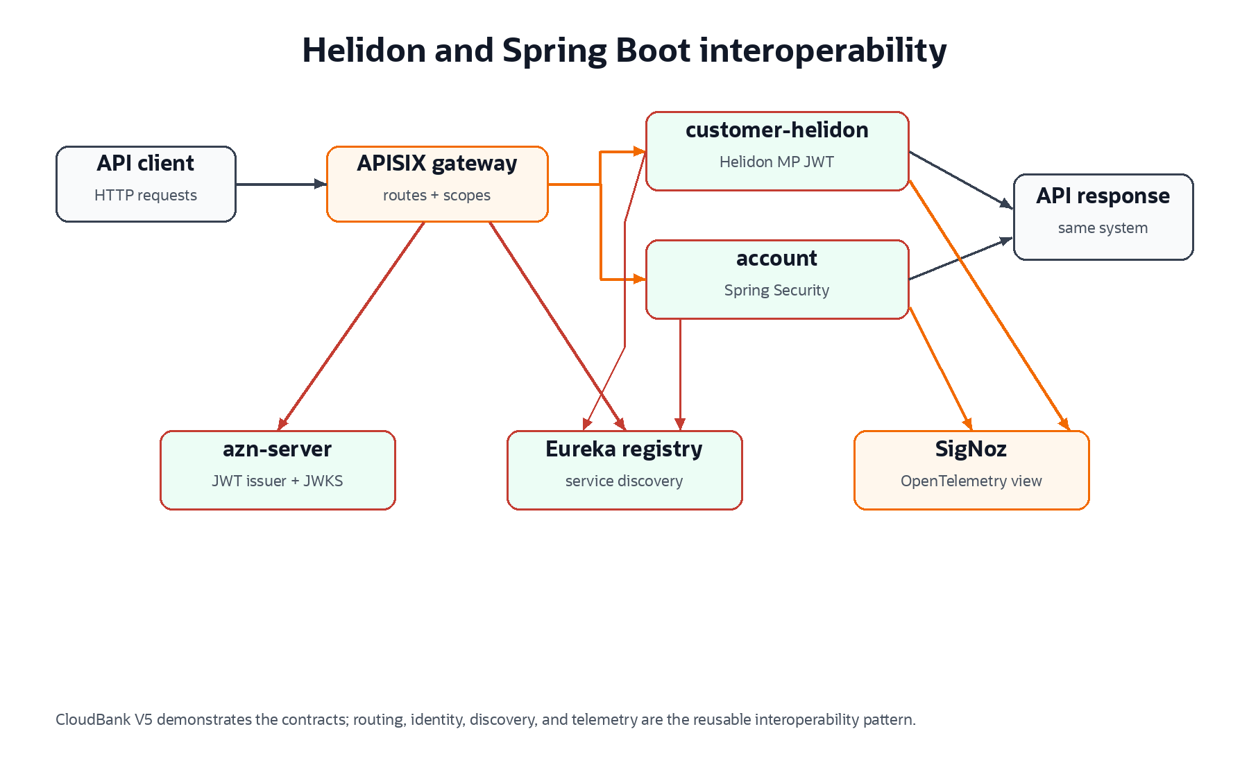
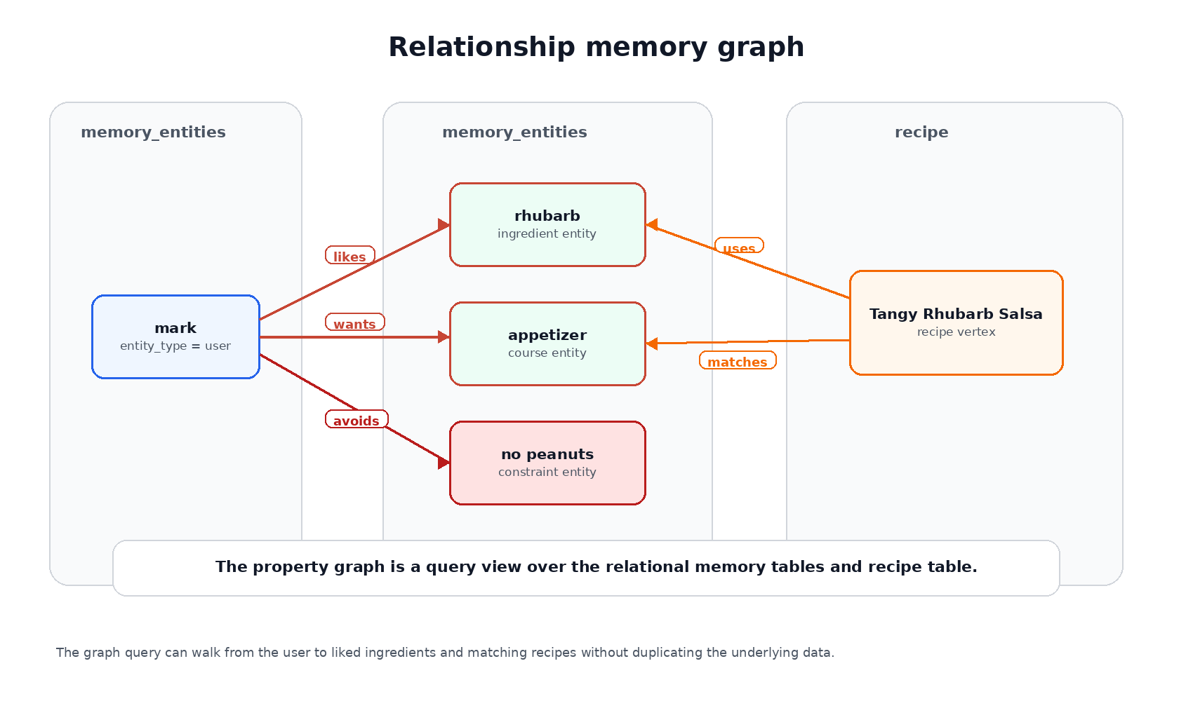
Before we move into vector retrieval, inspect the graph shape itself. The figure below uses circular vertices, labeled relationship pills, and connected edge property cards so the SQL graph definition is easier to connect to the query.
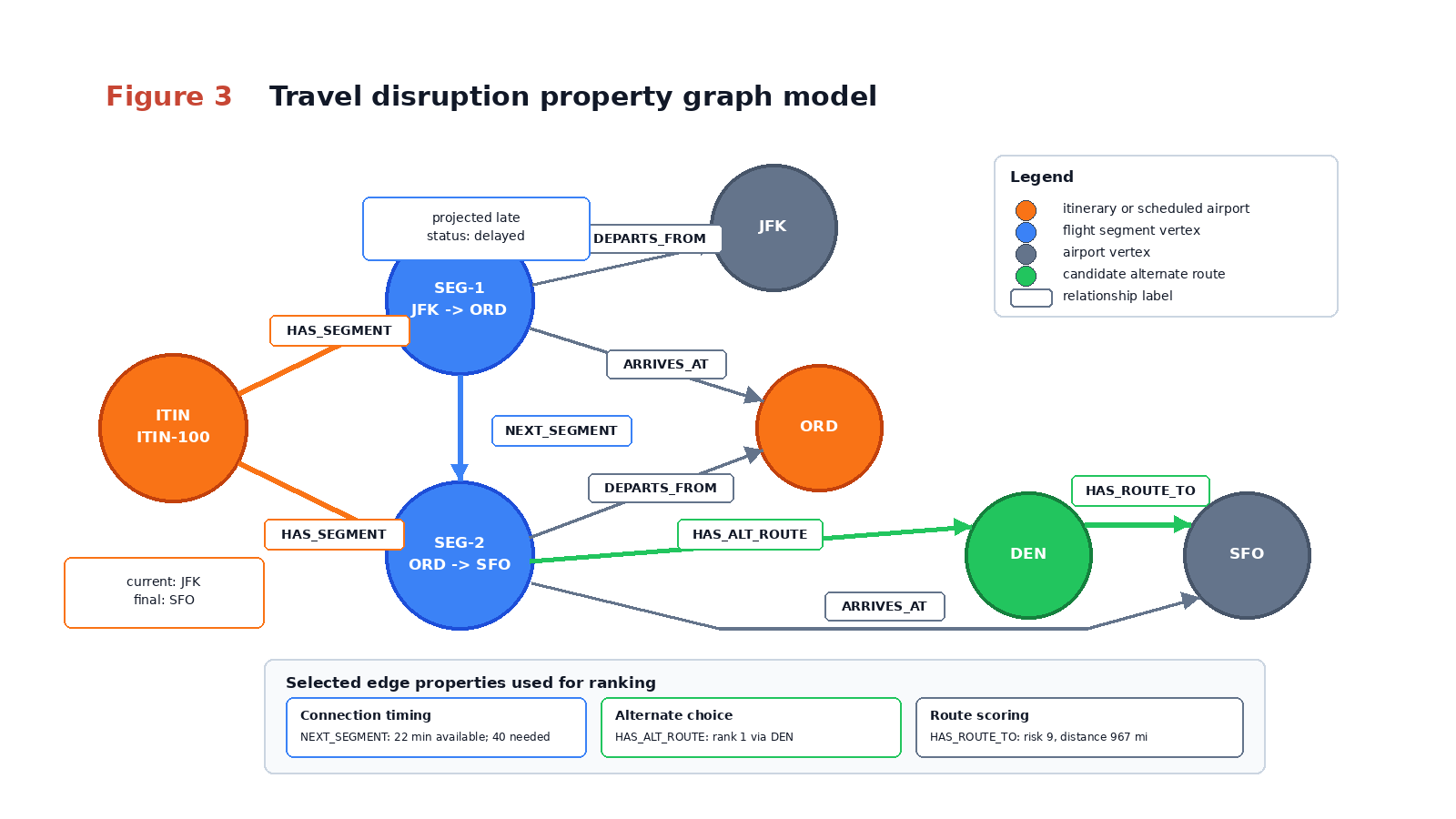
The route map earlier shows where the airports sit geographically. This model view shows what the database exposes to GRAPH_TABLE(): circular vertices are the things we traverse, relationship labels name the edges we follow, and the connected edge property cards show the evidence used to explain or rank the path.
Step 6: Embed policy chunks
Now generate policy embeddings with OpenAI and store them in policy_chunks.embedding.
python 06_embed_policy_chunks.py
The OpenAI provider wrapper keeps model calls out of the retrieval scripts. The retrieval scripts call a small interface instead of embedding provider code directly:
from openai_provider import OpenAIProviderprovider = OpenAIProvider(settings)vectors = provider.embed([content for _, _, content in common.POLICY_CHUNKS])
The wrapper is intentionally narrow:
class OpenAIProvider: def __init__(self, settings: Settings): self.settings = settings self.client = OpenAI(api_key=settings.openai_api_key) def embed(self, texts: Sequence[str]) -> list[list[float]]: # Use one embedding model for stored policy chunks and query vectors. response = self.client.embeddings.create( model=self.settings.openai_embedding_model, input=list(texts), ) vectors = [item.embedding for item in response.data] if not isinstance(vectors, list) or len(vectors) != len(texts): raise RuntimeError("OpenAI returned an invalid embedding payload") for vector in vectors: if len(vector) != self.settings.vector_dimension: raise RuntimeError("OpenAI embedding dimension does not match OPENAI_EMBEDDING_DIMENSION") return vectors
This keeps provider-specific code out of the retrieval path. The schema, graph query, and prompt builder only ask for embeddings or a generated answer. The dimension check is especially important because it catches a common vector bug before invalid rows are stored.
When the embedding script writes vectors, it converts Python floats into a database vector literal:
def vector_literal(values: Iterable[float]) -> str: return "[" + ",".join(f"{float(value):.8f}" for value in values) + "]"
That helper makes the handoff visible: the OpenAI provider returns Python lists of floats, and Oracle receives a serialized vector representation that this tutorial passes through TO_VECTOR() for readability. Before adapting the pattern for production or large loads, verify the current python-oracledb vector binding guidance for your driver and database version; a target environment may prefer a driver-native vector binding path.
Expected output:
Policy chunks embedded: 5Embedding dimension: <configured OPENAI_EMBEDDING_DIMENSION>
Oracle AI Database 26ai Free includes native vector support for this local lab, so no separate extension step is shown. We use VECTOR_DISTANCE() instead of shorthand vector distance operators such as <->, <=>, and <#> because the selected metric is visible in the SQL and easier for learners to inspect.
After embedding, a policy row has both readable text and a vector:
| policy_key | title | content excerpt | embedding shape |
|---|---|---|---|
| connection_buffer | Connection buffer | Use a minimum domestic connection buffer of 40 minutes… | VECTOR(<embedding dimension>, FLOAT32) |
| same_carrier_rebook | Same-carrier rebooking | For missed connections caused by delay… | VECTOR(<embedding dimension>, FLOAT32) |
The actual vector is a numeric array. The first few values are enough to show the shape:
[0.01234567,-0.09876543,0.22110000,0.00420000,...]
The numbers are not meant to be read one by one. What matters is that the policy chunks and the question use the same OpenAI embedding model and dimension, so Oracle can compare them with VECTOR_DISTANCE().
The small learning dataset has only a few policy chunks and intentionally does not create a vector index. For larger datasets, evaluate HNSW neighbor-graph indexes and IVF or IVFFlat neighbor-partition indexes with the current Oracle AI Vector Search documentation, your embedding dimension, your latency goals, and your recall requirements.
Advanced
Step 7: Compare retrieval modes
Run the comparison script to see what each retrieval mode can and cannot explain:
python 07_compare_retrieval_modes.py
Plain policy RAG can retrieve missed-connection policy language, but it cannot calculate the connection window. Hybrid vector plus relational retrieval can calculate the window and expose route scores. GraphRAG adds the connected path that explains why one alternative is better.
The comparison script is the main teaching tool in the demo. It does not ask the LLM which mode is better. It retrieves evidence for each mode and prints the missing pieces so you can see why graph-aware retrieval changes the answer.
The plain RAG query is only vector search over policy text:
SELECT title, contentFROM policy_chunksORDER BY VECTOR_DISTANCE(embedding, TO_VECTOR(:query_vector), COSINE)FETCH FIRST 2 ROWS ONLY
In Python, the query vector comes from the same OpenAI embedding path used for the stored policy chunks:
query_vector = common.vector_literal(provider.embed([QUESTION])[0])cur.execute( "SELECT title, content " "FROM policy_chunks " "ORDER BY VECTOR_DISTANCE(embedding, TO_VECTOR(:1), COSINE) " "FETCH FIRST 2 ROWS ONLY", [query_vector],)policy_rows = common.rows_to_dicts(cur)
The rows_to_dicts() helper turns cursor rows into dictionaries with lowercase column names. That makes later prompt construction explicit: the answer receives fields such as title, content, projected_buffer_minutes, and candidate_rank rather than anonymous tuple positions.
Representative result:
| rank | retrieved policy | what it can explain |
|---|---|---|
| 1 | Connection buffer | The rule, but not the itinerary timing |
| 2 | Same-carrier rebooking | The policy preference, but not the route path |
Mode B adds relational facts:
SELECT projected_buffer_minutes, required_buffer_minutesFROM segment_connect_edgesWHERE from_segment_id = 'SEG-1' AND to_segment_id = 'SEG-2'
The script then fetches the ranked alternative:
cur.execute( "SELECT airport_code, candidate_rank, route_risk_score, rationale " "FROM segment_alternative_route_edges " "WHERE segment_id = 'SEG-2' AND candidate_rank = 1")alternative = common.rows_to_dicts(cur)[0]
This intermediate mode proves that ordinary relational retrieval already solves part of the problem. You do not need graph traversal to know that 22 minutes is less than 40. You need graph traversal when you want to explain how the at-risk segment, the candidate airport, and the route evidence connect.
Representative result:
| projected_buffer_minutes | required_buffer_minutes | conclusion |
|---|---|---|
| 22 | 40 | connection is short by 18 minutes |
Mode C adds the graph path, which is why it can cite the connected alternative instead of merely saying “look for a rebooking.”
The graph retrieval follows the edges created from the helper tables. It starts at the disrupted outbound segment, follows the segment origin edge to ORD, traverses route summaries from ORD to DEN and DEN to SFO, and also checks that the segment has a ranked alternative edge to DEN:
cur.execute( "SELECT * FROM GRAPH_TABLE(travel_disruption_graph " "MATCH (seg IS segment)-[origin_edge IS departs_from]->(origin IS airport) " "-[first_leg IS has_route_to]->(mid IS airport) " "-[second_leg IS has_route_to]->(dest IS airport), " "(seg)-[alt IS has_alternative_route]->(mid) " "WHERE seg.segment_id = 'SEG-2' " "AND origin.airport_code = 'ORD' " "AND mid.airport_code = 'DEN' " "AND dest.airport_code = 'SFO' " "COLUMNS (" "seg.segment_id AS disrupted_segment, " "origin.airport_code AS origin_airport, " "mid.airport_code AS alternative_connection_airport, " "dest.airport_code AS destination_airport, " "alt.candidate_rank AS candidate_rank, " "alt.route_risk_score AS candidate_route_risk_score, " "first_leg.route_risk_score AS first_leg_route_risk_score, " "second_leg.route_risk_score AS second_leg_route_risk_score" ")) ORDER BY candidate_rank")alternative_path = common.rows_to_dicts(cur)
This is where the demo moves from “retrieve some rows” to “retrieve a connected explanation.” The graph path proves SEG-2 -> ORD -> DEN -> SFO, while the alternative edge proves that DEN is the ranked candidate midpoint for the disrupted segment. The edge properties carry rank and route scores, so the answer summarizes retrieved evidence instead of inventing a reroute.
| mode | evidence retrieved | answer quality |
|---|---|---|
| Plain RAG | policy chunks | generic policy answer |
| Hybrid vector + relational | policy chunks plus buffer row | specific “no,” but route path is manual |
| GraphRAG | policy chunks, buffer row, graph path | specific “no” plus DEN alternative path |
Representative output:
Mode A evidence: policy chunks onlyMode B evidence: policy chunks + itinerary timing + route summariesMode C evidence: policy chunks + itinerary timing + graph path + alternativesRecommended mode: C
The exact vector distances can vary with the supplied embedding model. The important comparison is the evidence coverage, not a hard-coded score.
The script also includes a tiny query router:
def route_question(question: str) -> list[str]: lowered = question.lower() modes: list[str] = [] if any(term in lowered for term in ["policy", "missed connection", "caused by"]): modes.append("vector") if any(term in lowered for term in ["connection", "alternative", "route", "itinerary", "risk", "path"]): modes.append("graph") if not modes: modes.append("vector") return modes
This router is intentionally basic. Its purpose is to show the retrieval design decision, not to solve natural-language routing. Policy questions can use vector retrieval. Questions about connection risk, alternatives, route paths, or itinerary structure need graph evidence. A production implementation might replace this with a tested classifier, but the principle is the same: choose retrieval tools based on the evidence needed to answer safely.
Step 8: Generate the grounded answer
Finally, generate the passenger-facing answer from Mode C evidence:
python 08_answer_question.py
Representative answer:
You are unlikely to make the current connection. The projected arrival at ORD leaves less than the demo 40-minute connection buffer before the ORD to SFO departure. The ranked tutorial alternative is ORD to DEN to SFO because the demo graph connects the at-risk segment to DEN and the candidate score is computed from the staged route summaries.
The answer includes an explanation path:
Passenger itinerary -> inbound segment JFK to ORD -> projected arrival delay -> connection at ORD -> required connection buffer -> outbound segment ORD to SFO -> alternative route ORD to DEN to SFO -> policy chunk: same-carrier rebooking
The answer script builds the prompt from retrieved evidence, not from the user’s question alone:
prompt = f"""Answer with grounded travel disruption guidance only.Use these headings exactly: Recommendation, Connection feasibility, Evidence path,Policy basis, Alternatives considered, Confidence and caveat, Data freshness disclaimer.Use only supplied graph facts, relational facts, and policy chunks. If evidence is missing,say what is missing.Question: {QUESTION}Projected buffer: {connection["projected_buffer_minutes"]} minutesRequired buffer: {connection["required_buffer_minutes"]} minutesAlternative: {alternative["airport_code"]} - {alternative["rationale"]}Policies: {policy_rows}Graph evidence: {graph_rows}State that this is tutorial data, not real-time operational airline advice."""answer = provider.generate(prompt)
The headings force the generated answer to separate recommendation, feasibility, evidence, policy basis, alternatives, confidence, and data freshness so reviewers can spot unsupported advice.
The generation method uses the same narrow OpenAI wrapper as embeddings:
def generate(self, prompt: str) -> str: response = self.client.responses.create(model=self.settings.openai_model, input=prompt) text = response.output_text if not isinstance(text, str) or not text.strip(): raise RuntimeError("OpenAI returned an empty generation result") return text.strip()
That keeps the tutorial focused on GraphRAG rather than provider plumbing. The rest of the code only knows that the provider can embed text and generate grounded text.
Run the static validator and optional cleanup when finished:
python 09_validate_demo.pypython 10_cleanup_demo.py
The validator checks file presence, syntax, credential hygiene, local Compose setup, init SQL, and static project consistency. Live database execution uses the included Oracle AI Database 26ai Free container plus your OpenAI configuration.
Tips And Troubleshooting
Keep the tutorial schema small while learning the pattern. It is easier to inspect a six-airport graph than to debug a full operational feed before the retrieval modes are clear.
Use environment variables for all credentials and model identifiers. The demo package’s .env.example is intentionally placeholder-only, and the scripts should never print passwords, tokens, wallet contents, or private endpoint values.
When graph creation fails, check that the helper edge tables are populated and that the source and destination keys reference the intended vertex tables. The tutorial graph deliberately avoids using the same relational table as both a vertex table and an edge table in the same relationship.
When vector results look surprising, inspect the retrieved doc_name, chunk_title, and distance values before changing prompts. For a larger policy corpus, add indexing only after validating the embedding model, vector dimension, metric, and expected recall behavior.
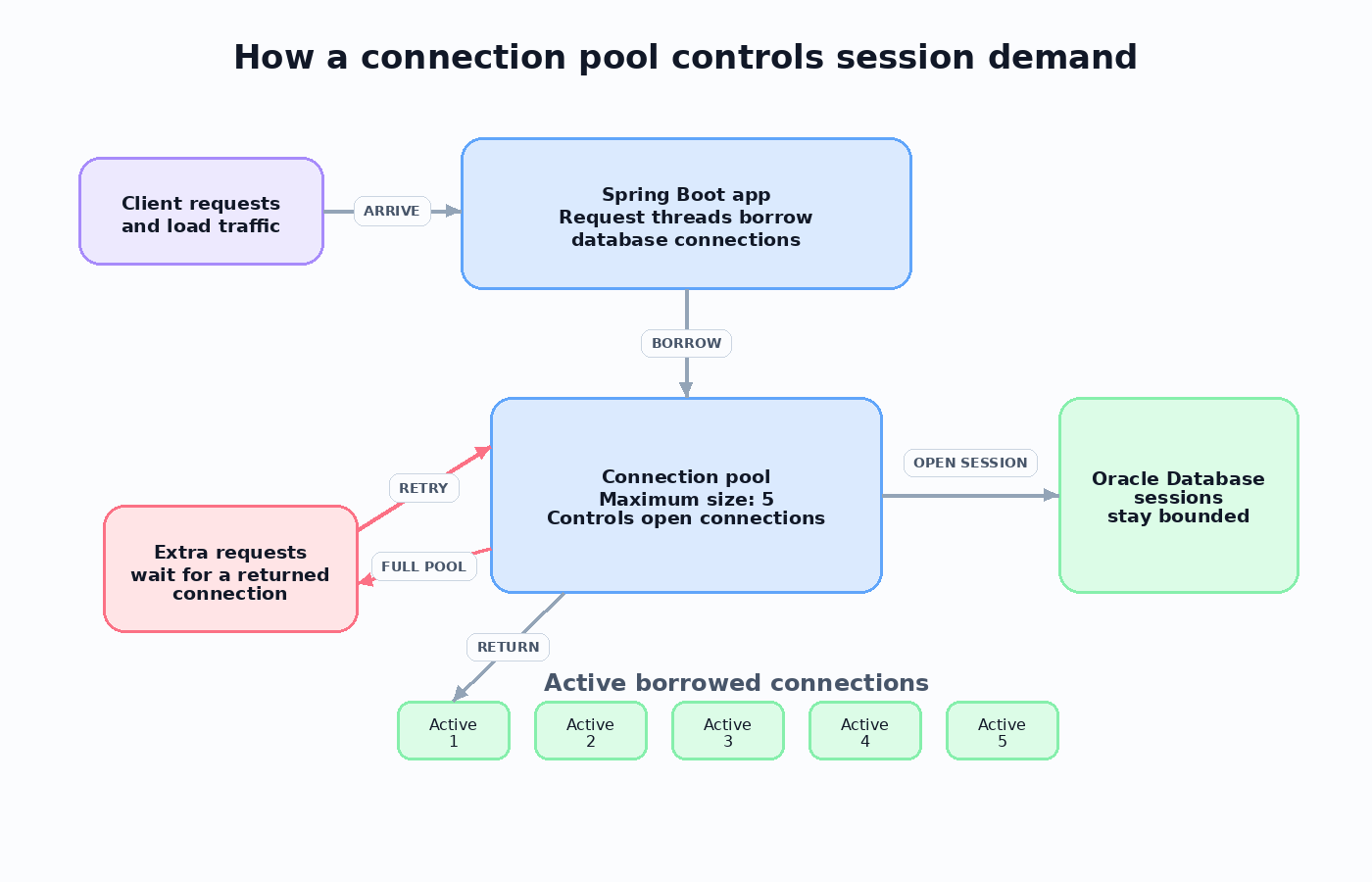
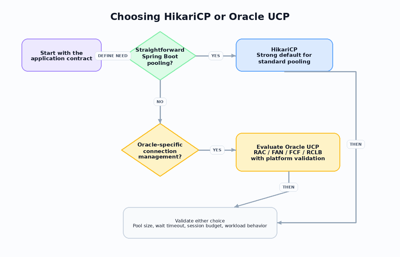
For production services, create a python-oracledb connection pool with oracledb.create_pool() instead of opening one connection per question. Batch embedding calls where your OpenAI rate limits and latency goals support batching, and monitor cost, rate limits, and latency before scaling bulk loads or query fan-out.
Telemetry is optional for this tutorial run. If your environment emits spans to shared infrastructure, keep attributes free of secrets and treat delivery confirmation as operational evidence rather than a prerequisite for understanding the GraphRAG pattern.
Oracle AI Vector Search Notes
This tutorial uses the included Oracle AI Database 26ai Free Compose setup for local execution. The mounted init SQL creates a least-privilege graphrag_demo user in FREEPDB1; the Python checkpoints then create only application-owned tutorial objects.
Oracle AI Database 26ai-compatible environments include native support for the VECTOR data type and VECTOR_DISTANCE(). If you adapt the demo to another environment, keep the runtime user least-privilege and verify the vector and SQL property graph features before running the checkpoints.
The demo uses small deterministic vectors so every ranking step is inspectable. In production, keep vector generation provider-configurable: use the approved embedding provider or embedding API for the environment, and generate document vectors and query vectors with the same embedding model so their vector dimensions and distance relationships are comparable.
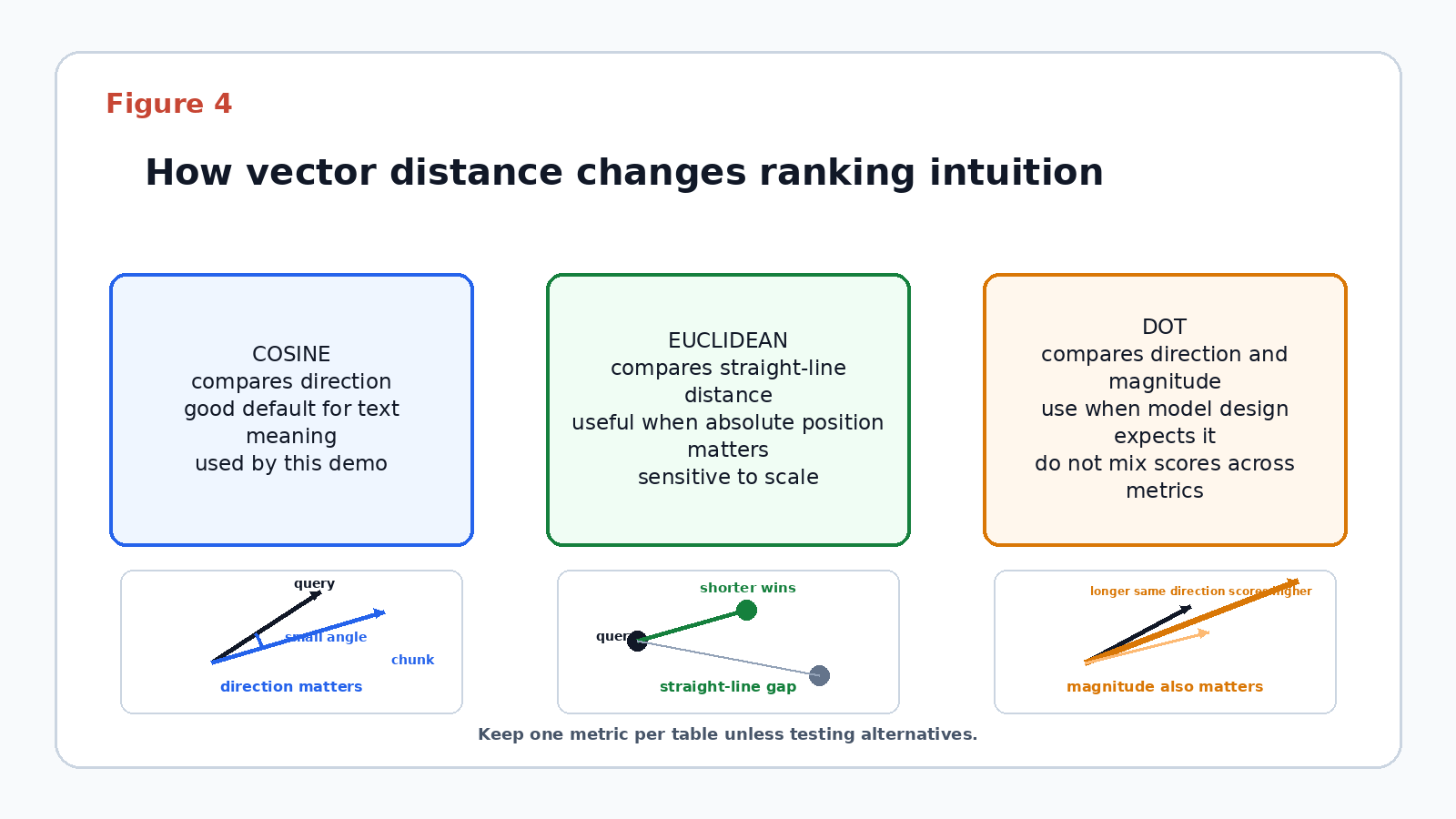
Metric choice depends on the embedding model and scoring goal: cosine is useful when vector direction matters more than magnitude, Euclidean is useful when absolute distance and vector magnitude are meaningful, and dot-product-style scores are useful only when the model and normalization strategy make score direction explicit.
For larger datasets, evaluate vector index choices in the target environment. HNSW indexes are a good fit when recall and low-latency nearest-neighbor lookups matter and additional memory is acceptable. IVF or IVFFlat-style neighbor partition indexes are useful when partitioned search and memory control are more important. The right choice depends on workload size, latency goals, recall goals, and metric alignment.
This tutorial keeps the runnable lab focused on the small policy_chunks table and does not publish exact vector-index DDL. Before adding an index example to production documentation, validate the current Oracle AI Vector Search syntax in the target environment and use table names from the real schema being documented.
Conclusion
We built a travel disruption assistant that shows why GraphRAG matters for connected questions. Plain policy retrieval finds relevant words, hybrid retrieval adds structured facts, and the graph-aware mode supplies the path that ties the passenger, flights, airports, connection buffer, route alternatives, and policy evidence together.
This pattern fits applications where the answer depends on both semantic text and explainable relationships. It is not a substitute for validated operational systems, live airline data, or production decision policies. The next useful step is to run the extracted local demo, inspect the Mode A/B/C evidence side by side, and then adapt the schema to one additional connected scenario.
Related resources:
- Oracle AI Database – Start with the database platform used for the relational, vector, and graph portions of the lab.
- Oracle AI Vector Search LiveLabs – Continue with hands-on workshops for hybrid search, RAG, and chatbot retrieval patterns.
- Oracle Graph documentation – Review SQL property graph concepts and graph query options.
- Python-oracledb documentation – Use the Python driver reference when adapting connection, bind, and transaction handling.
- Bureau of Transportation Statistics TranStats – Explore the historical flight performance source that inspired the staged tutorial fields.


You must be logged in to post a comment.