If you have ever asked, “How is this thing connected to that thing?”, you have already asked a graph question.

A customer sends money to an account. That account sends money to two other accounts. One of those accounts sends money back to the original customer. In ordinary SQL, you can query each transfer. But when the real question is about chains, loops, hubs, and hidden intermediaries, the shape of the question becomes graph-shaped.

Oracle AI Database 26ai makes that graph shape part of the database instead of a separate side project. You can model a property graph over existing relational tables, query it with SQL graph syntax, join the results back to relational data, and then move into Graph Studio or PGX when you need visualization or heavier analytics.

Did you know that graphs were added to the SQL standard? Read about it here.

This series starts from zero. You do not need graph theory. You do not need a separate graph database. You need a basic comfort with SQL and a practical problem where relationships matter.

There are two ways you can try the runnable examples in this series. The first path is to use FreeSQL and this will work just fine for most of the examples: creating the tables, creating the graph, and querying patterns with GRAPH_TABLE. The second path is your own Autonomous Database Serverless instance on OCI for the full analytics chapter, because the DBMS_OGA algorithm examples require packages that are not available in the FreeSQL environment.

By the end of this article, you should be able to explain five ideas well enough to understand the graph DDL in the next article: vertex, edge, label, property, and directed relationship. You should also understand why Oracle’s 26ai graph approach is accessible from ordinary SQL instead of starting in a separate graph-only tool.

That is the only conceptual load for now. We will save weighted paths, algorithms, PGX, and natural-language querying for later articles, when those ideas have a working graph underneath them.

The Graph Mental Model

A graph has two main parts: vertices and edges.

A vertex is a thing. In a banking example, a vertex might be an account. In a social network, it might be a person. In a supply chain, it might be a warehouse, supplier, shipment, or part.

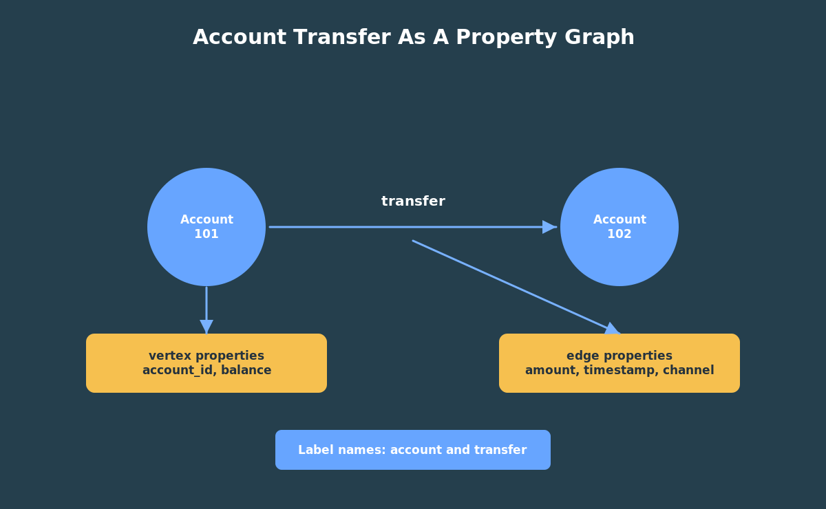
An edge is a relationship between things. In the banking example, a transfer from account 101 to account 102 is an edge. The edge has direction because money moved from one account to another.

Both vertices and edges can have properties. An account vertex can have an account id, customer id, account name, and balance. A transfer edge can have an amount, timestamp, channel, and note.

Labels give those things names in the graph model. In this series, account vertices use the label account, and transfer edges use the label transfer. Labels make graph patterns readable because you can ask for accounts connected by transfers instead of thinking only in table and column names.

That gives us a simple model:

• account is a vertex;
• transfer is an edge;
• transfer direction goes from source account to destination account;
• transfer amount and timestamp are edge properties;
• customer id and balance are vertex properties.

The point is not to replace tables. The point is to describe relationships over data you already have.

That distinction helps avoid a common beginner mistake. You are not deciding whether the account data is “relational” or “graph.” It is relational data that also has a graph interpretation. Oracle lets you keep both views of the same facts.

Why Graph Questions Feel Different

Relational databases are excellent at storing and querying structured facts. A transfer table can tell you that account 101 sent 500 dollars to account 102. A customer table can tell you that account 102 belongs to a medium-risk customer.

Graph questions start when the relationship pattern matters.

For example:

• Which accounts receive money from many different sources?
• Which accounts sit in the middle of two-hop transfer chains?
• Which accounts participate in round-trip transfer cycles?
• Which high-risk customers are connected to suspicious paths?

You can answer some of these with ordinary joins, especially when the path length is fixed and short. But the queries become harder to read as soon as you want to ask about paths, cycles, or repeated relationship patterns.

That is where GRAPH_TABLE becomes useful. It lets you describe a graph pattern and return the matches as rows. Once the graph match is back in row form, you can use normal SQL again: filter it, aggregate it, join it, and sort it.

What Changed In 26ai

In Oracle AI Database 26ai, SQL property graphs are native database objects. You create them with CREATE PROPERTY GRAPH, and you query them with SQL graph syntax such as GRAPH_TABLE.

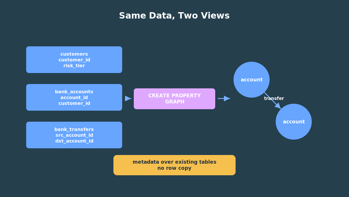
The important beginner idea is this: a SQL property graph is metadata over database objects. You do not have to copy all of your rows into a separate graph store just to start asking graph questions. The graph definition says which tables provide vertices, which tables provide edges, how the keys connect, which labels to use, and which properties to expose.

For the bank example in this series, the relational data is still stored in ordinary tables:

• customers
• bank_accounts
• bank_transfers

The graph object simply gives those tables graph meaning:

• bank_accounts becomes account vertices;
• bank_transfers becomes transfer edges;
• src_account_id and dst_account_id define edge direction.

That is why graph in 26ai is a good fit for developers and DBAs who already work with Oracle Database. You can start with SQL, keep the data where it is, and add graph-shaped queries where they help.

Why Not RDF?

Oracle supports RDF graphs too, but this series is about property graphs. RDF is the better fit when the work centers on formal semantics, ontologies, inferencing, and standards-based knowledge representation. Property graphs are the better starting point here because the question is operational and concrete: how are these accounts connected, and what suspicious patterns do those connections form?

The Bank Fraud Story We Will Use

The rest of this series uses a small bank-fraud style example. It is intentionally tiny so you can understand every row.

The demo has customers, accounts, and transfers. Some transfers form a simple cycle. Other transfers create a fan-in pattern where several accounts send money to the same destination. Another chain places a high-risk customer in the middle.

That gives us enough data to teach useful graph ideas without hiding the lesson inside a huge dataset.

Here is the shape of the data we will use throughout this series:

customers      bank_accounts      bank_transfers
----------     -------------      --------------
customer_id -> customer_id        transfer_id
risk_tier      account_id      -> src_account_id
               account_name    -> dst_account_id
               balance            amount
                                  transfer_ts
                                  channel

The SQL property graph gives those tables this connected shape:

(account)-[transfer]->(account)

That one pattern, account connected to account by transfer, is enough to teach all four articles’ worth of graph concepts: paths, cycles, hubs, chains, ranking, connected groups, and hybrid SQL joins.

Where This Series Is Going

The next article builds the graph. We will create the tables, load seed data, define BANK_GRAPH, and inspect the graph metadata.

After that, we will query fraud patterns with GRAPH_TABLE. Then, in ADB-S, we will add in-database algorithms with DBMS_OGA and use Graph Studio to visualize the same graph.

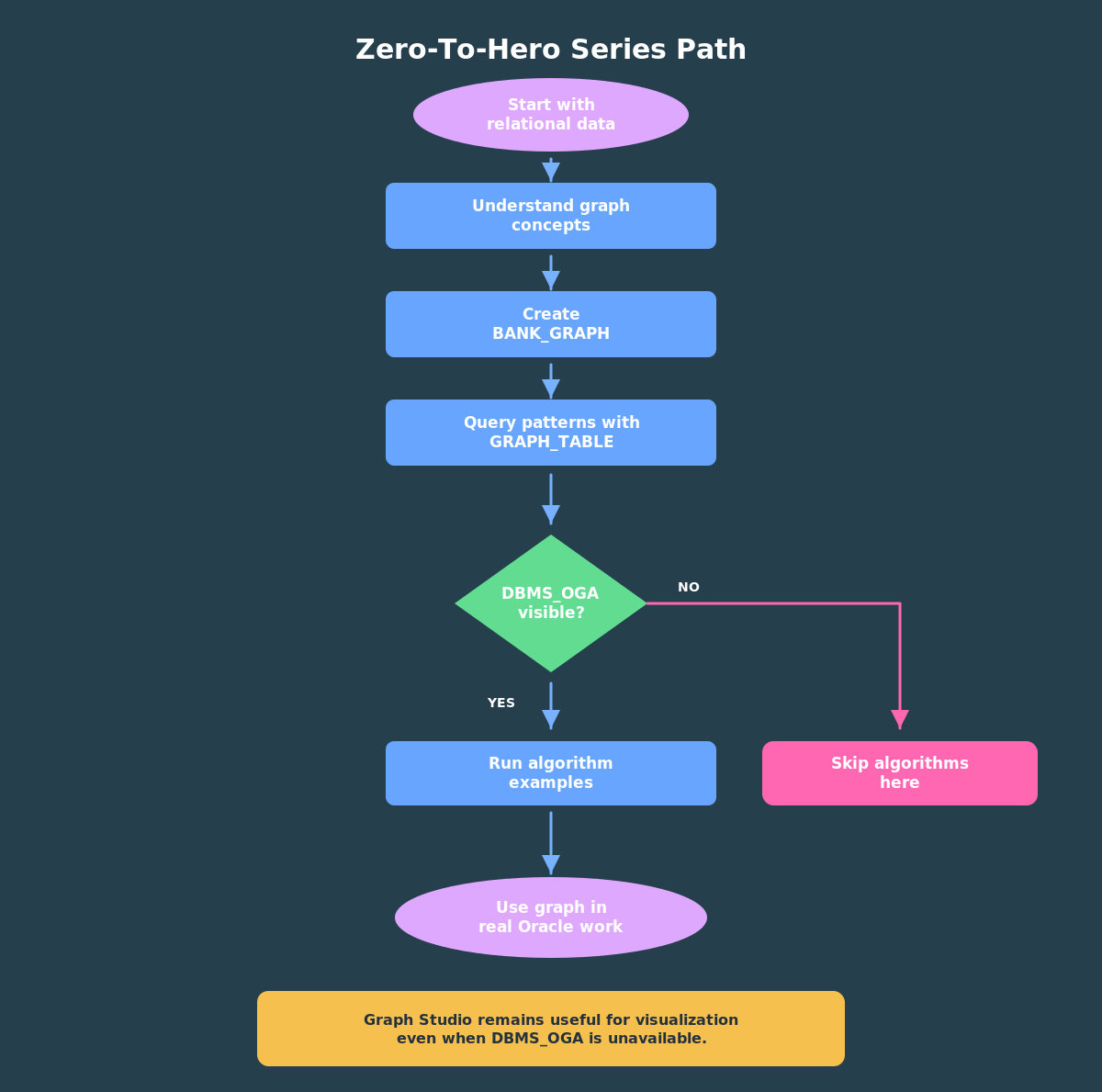
The goal is not to memorize every graph feature. The goal is to build a practical mental model:

1. start with relational data;
2. define a SQL property graph;
3. query graph patterns with SQL;
4. join graph results to ordinary data;
5. move into Graph Studio or PGX when you need visualization or deeper analytics.

That is the zero-to-hero path.

Try The Demo

The fastest way to make the ideas concrete is to run the tiny bank demo yourself. The first runnable step creates three ordinary relational tables:

• customers
• bank_accounts
• bank_transfers

Those tables hold the facts. The next step creates BANK_GRAPH, a SQL property graph over the account and transfer rows. Nothing is copied into a separate graph store; the graph definition gives the existing rows a connected shape.

Note: this will ask you to login with your oracle.com account since it writes to the database, not just reads. It’s totally free. I recommend you read through the SQL first to understand what it does, then click on the “Run Script” button to execute it, and then scroll through the output to see what happened. Feel free to play around with it and change it however you like!

In the next article, you’ll load the seed data and create the graph. If you prefer to use your own Autonomous Database Serverless instance, copy the same SQL into your SQL Worksheet and run it there. Either way, keep the data small at first. The goal is to see the graph model clearly before adding larger datasets, algorithms, or visualization.

Once BANK_GRAPH exists, the later examples will use the same graph to find inbound hubs, transfer chains, cycles, PageRank scores, connected groups, and weighted paths.