
Key Takeaways
- Vector RAG is useful for semantic recall, but relationship-heavy questions can be harder to inspect when evidence is spread across chunks.
- GraphRAG adds explicit entities, relationships, confidence scores, and evidence links so relationship-heavy retrieval can be inspected and cited.
- Oracle AI Database 26ai can store the relational tables,
VECTORembeddings, extracted graph rows, and SQL property graph metadata used in a database-centered GraphRAG workflow. - This walkthrough compares baseline vector retrieval, graph-enriched chunk embeddings, and an Oracle SQL hybrid query over the first 500 usable rows from a larger, entity-rich corpus.
Standard vector Retrieval-Augmented Generation, or RAG, retrieves chunks that are semantically similar to a question. That works well when the answer appears in a compact passage whose wording is close to the question. It becomes harder to inspect when the answer depends on relationships among people, places, organizations, events, objects, or concepts scattered across several chunks.
A relationship-heavy question shows the problem:
Which documents connect this person, organization, place, and event, and what evidence supports that connection?
A plain vector retriever may return chunks about one entity, chunks about another entity, or chunks about the general topic. Those chunks may be useful, but vector similarity alone does not give us an inspectable fact such as “this person is connected to this organization through this event, supported by this sentence in this chunk.”
GraphRAG adds that missing relationship layer. In this tutorial, we build a GraphRAG pipeline with Oracle AI Database 26ai. We parse and chunk the first 500 usable rows from a larger Kaggle-style corpus with Docling, extract entities and relationships automatically, store the results in relational tables, define a SQL property graph, generate raw and graph-enriched embeddings, and compare three retrieval paths:
- baseline vector retrieval over raw chunks;
- vector retrieval over graph-enriched chunks;
- an Oracle SQL hybrid query that uses graph evidence and vector distance in the same SQL statement.
The goal is not to prove universal graph superiority over vector search. GraphRAG adds extraction, entity resolution, graph maintenance, scoring, and evaluation work. The practical question is narrower: when graph context helps, where should it enter the retrieval path?
The Architecture
GraphRAG combines semantic retrieval with graph-structured retrieval. The graph is useful only if every extracted fact can be traced back to source evidence.
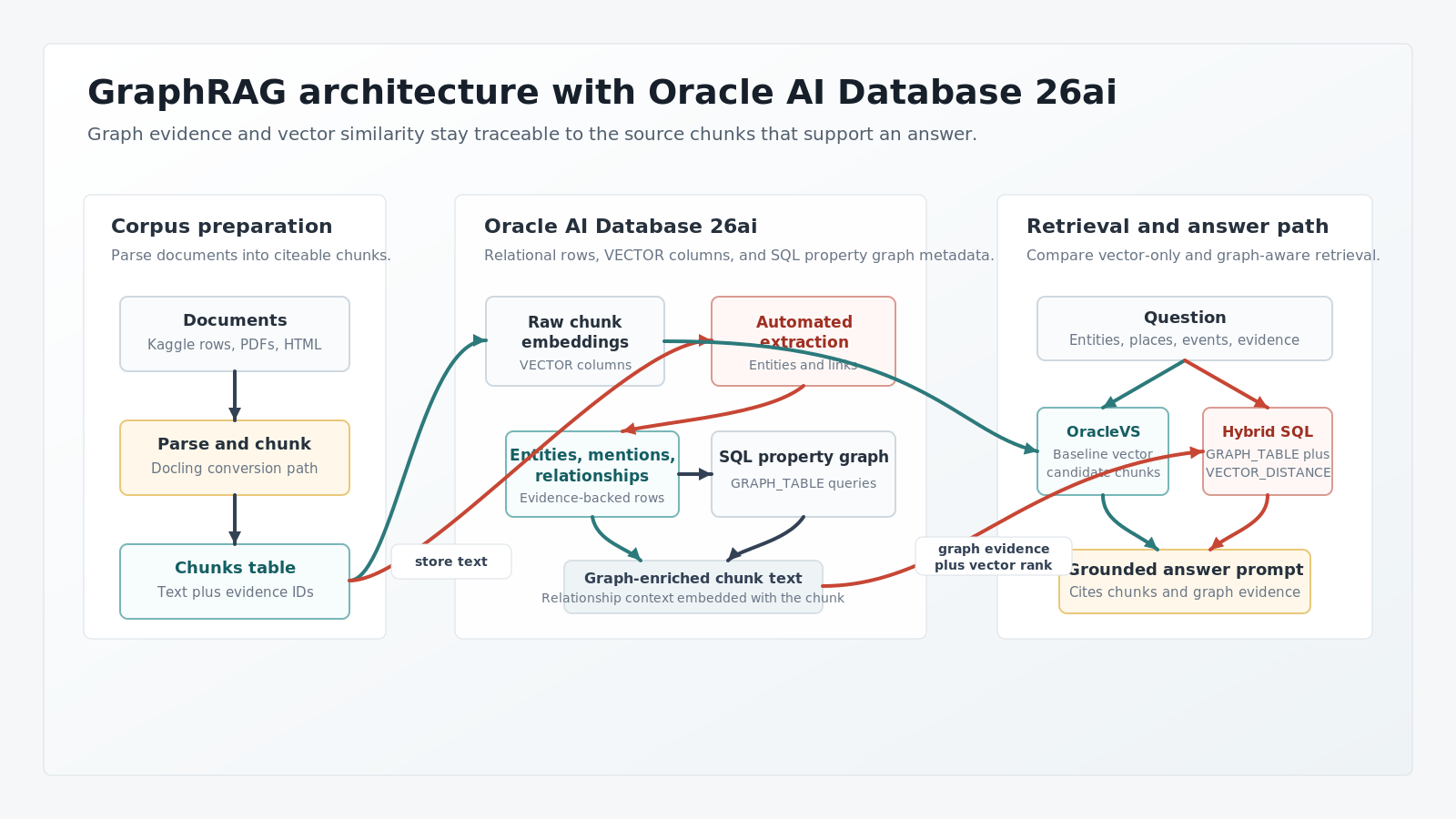
Oracle AI Database 26ai provides the database pieces used here: relational tables, VECTOR columns, VECTOR_DISTANCE, SQL property graphs created with CREATE PROPERTY GRAPH, and graph pattern queries through GRAPH_TABLE.
Useful source anchors:
- Oracle AI Database 26ai docs: https://docs.oracle.com/en/database/oracle/oracle-database/26/
VECTORdata type: https://docs.oracle.com/en/database/oracle/oracle-database/26/vecse/create-tables-using-vector-data-type.htmlVECTOR_DISTANCE: https://docs.oracle.com/en/database/oracle/oracle-database/26/vecse/vector_distance.htmlCREATE PROPERTY GRAPH: https://docs.oracle.com/en/database/oracle/oracle-database/26/sqlrf/create-property-graph.html- Graph reference for
GRAPH_TABLE: https://docs.oracle.com/en/database/oracle/oracle-database/26/sqlrf/graph-reference.html - python-oracledb vector support: https://python-oracledb.readthedocs.io/en/latest/user_guide/vector_data_type.html
This article uses SQL property graphs as the main graph path, rather than the older in-memory graph tooling path.
Dataset And Environment
Use a larger entity-rich corpus instead of a hand-sized literary sample. A good fit for this tutorial is a Kaggle corpus of plot summaries or article abstracts where each row contains a title, text body, and metadata that can be cited. One practical candidate is the Kaggle Wikipedia Movie Plots-style corpus, because movie plots contain people, places, organizations, events, objects, and relationship-heavy narrative arcs. Use it only when the dataset page shows a license that allows reuse in tutorial content, and carry the required attribution into the sample repository. If your Kaggle workspace shows a different license, choose another Kaggle corpus with a permissive or clearly documented reuse license before publishing.
The snippets assume an Oracle AI Database 26ai environment where your user can create VECTOR columns, create SQL property graphs, and query them with VECTOR_DISTANCE and GRAPH_TABLE. Oracle AI Database 26ai Free, Autonomous AI Database Free, and FreeSQL-style sandboxes can be useful for demos, but verify privileges, resource limits, remote connectivity, and vector index support in the exact target environment before running the 500-row workflow.
Install the Python packages used by the snippets:
python -m pip install oracledb pandas python-dotenv docling gliner langchain langchain-community==0.3.31 langchain-huggingface sentence-transformers
The OracleVS import used later in this article was validated with langchain-community==0.3.31. In the current 0.4.x package line, that integration is no longer available at langchain_community.vectorstores.oraclevs, so pin the dependency for this sample or update the baseline retriever to the replacement integration available in your environment.
This demo uses the Oracle AI Database 26ai Free container, exposed locally as localhost:1522/FREEPDB1, or another host port mapped to the container’s FREEPDB1 service. For that local container path, create a dedicated application schema in an automatic segment space management tablespace. Do not let the demo user default to SYSTEM; VECTOR columns cannot be created in the non-ASSM SYSTEM tablespace in the validated local container. For large direct path loading tests, use the full Free container image rather than a reduced lite image if the lite image omits dictionary components required by direct path load.
Run the following as an administrative user connected to FREEPDB1, adapting the datafile path if your container stores PDB datafiles somewhere else:
CREATE TABLESPACE graphrag_data DATAFILE '/opt/oracle/oradata/FREE/FREEPDB1/graphrag_data01.dbf' SIZE 500M AUTOEXTEND ON NEXT 100M MAXSIZE 5G SEGMENT SPACE MANAGEMENT AUTO;CREATE USER graphrag_app IDENTIFIED BY "replace-with-a-strong-password" DEFAULT TABLESPACE graphrag_data QUOTA UNLIMITED ON graphrag_data;GRANT CREATE SESSION TO graphrag_app;GRANT CREATE TABLE TO graphrag_app;GRANT CREATE VIEW TO graphrag_app;GRANT CREATE SEQUENCE TO graphrag_app;GRANT CREATE PROCEDURE TO graphrag_app;GRANT CREATE PROPERTY GRAPH TO graphrag_app;
Then set the application connection variables:
export ORACLE_USER=graphrag_appexport ORACLE_PASSWORD="replace-with-a-strong-password"export ORACLE_DSN="localhost:1521/FREEPDB1"
The embedding examples use sentence-transformers/all-MiniLM-L6-v2, which produces 384-dimensional dense embeddings and is published under the Apache-2.0 license:
https://huggingface.co/sentence-transformers/all-MiniLM-L6-v2
That model choice is why the table below uses VECTOR(384, FLOAT32). If you change embedding models, change the vector dimension and rebuild embeddings and indexes.
Parse And Chunk The Corpus With Docling
Docling should be part of the runnable path, not just a future suggestion. For CSV-based Kaggle datasets, convert selected rows into small Markdown documents, then let Docling perform document conversion so the pipeline uses the same parser abstraction you would use for PDFs, DOCX, HTML, and other enterprise document formats.
Docling reference: https://docling-project.github.io/docling/
The following setup turns the first 500 usable rows of a Kaggle-style CSV into Docling-readable Markdown files. Adapt the column names to the dataset you choose. In the validated local run, those 500 rows produced 1,155 chunks and the full workflow completed in about 6 minutes on the test machine.
from dataclasses import dataclassfrom pathlib import Pathimport reimport textwrapimport pandas as pdfrom docling.document_converter import DocumentConverterDATASET_CSV = Path("data/wiki_movie_plots_deduped.csv")DOC_DIR = Path("work/docling_input")MAX_DOCUMENTS = 500 # Keep the tutorial run bounded and repeatable.WORDS_PER_CHUNK = 220dataclassclass Chunk: document_key: str document_title: str section_title: str chunk_index: int chunk_text: strdef normalize_space(text: str) -> str: return re.sub(r"s+", " ", str(text)).strip()def write_markdown_documents(csv_path: Path, output_dir: Path, limit: int) -> list[Path]: output_dir.mkdir(parents=True, exist_ok=True) frame = pd.read_csv(csv_path).dropna(subset=["Title", "Plot"]) frame = frame.head(limit) paths = [] for index, row in frame.iterrows(): title = normalize_space(row["Title"]) plot = normalize_space(row["Plot"]) year = normalize_space(row.get("Release Year", "")) origin = normalize_space(row.get("Origin/Ethnicity", "")) genre = normalize_space(row.get("Genre", "")) path = output_dir / f"movie_{index:05d}.md" path.write_text( textwrap.dedent( f""" # {title} Release year: {year} Origin: {origin} Genre: {genre} ## Plot {plot} """ ), encoding="utf-8", ) paths.append(path) return pathsdef chunk_words(document_key: str, title: str, section: str, text: str) -> list[Chunk]: words = normalize_space(text).split() chunks = [] for chunk_index, start in enumerate(range(0, len(words), WORDS_PER_CHUNK), start=1): chunk = " ".join(words[start:start + WORDS_PER_CHUNK]) if chunk: chunks.append(Chunk(document_key, title, section, chunk_index, chunk)) return chunksdef docling_chunks(paths: list[Path]) -> list[Chunk]: converter = DocumentConverter() chunks = [] for path in paths: result = converter.convert(path) markdown = result.document.export_to_markdown() title = path.stem heading = markdown.splitlines()[0].lstrip("# ").strip() if markdown else path.stem chunks.extend(chunk_words(path.stem, heading, "plot", markdown)) return chunksdocument_paths = write_markdown_documents(DATASET_CSV, DOC_DIR, MAX_DOCUMENTS)all_chunks = docling_chunks(document_paths)print(f"Prepared {len(all_chunks)} chunks from {len(document_paths)} documents")
Keep the tutorial default at 500 rows. The complete dataset can be useful for stress testing, but it is too slow for a normal article walkthrough. In the validated 500-row run, the script reported:
DOCLING_OK documents=500 chunks=1155
Create The Oracle Tables
The relational schema keeps chunks, entities, relationship evidence, and embeddings separate. That separation matters because it lets us compare retrieval strategies without changing the source corpus.
CREATE TABLE documents ( document_id NUMBER GENERATED BY DEFAULT AS IDENTITY PRIMARY KEY, title VARCHAR2(400) NOT NULL, source_url VARCHAR2(1000), license_note VARCHAR2(1000));CREATE TABLE chunks ( chunk_id NUMBER GENERATED BY DEFAULT AS IDENTITY PRIMARY KEY, document_id NUMBER NOT NULL REFERENCES documents(document_id), section_title VARCHAR2(400), chunk_index NUMBER NOT NULL, chunk_text CLOB NOT NULL, CONSTRAINT chunks_uq UNIQUE (document_id, section_title, chunk_index));CREATE TABLE entities ( entity_id NUMBER GENERATED BY DEFAULT AS IDENTITY PRIMARY KEY, canonical_name VARCHAR2(400) NOT NULL, entity_type VARCHAR2(64) NOT NULL, aliases_json CLOB CHECK (aliases_json IS JSON), confidence NUMBER, CONSTRAINT entities_uq UNIQUE (canonical_name, entity_type));CREATE TABLE entity_mentions ( mention_id NUMBER GENERATED BY DEFAULT AS IDENTITY PRIMARY KEY, entity_id NUMBER NOT NULL REFERENCES entities(entity_id), chunk_id NUMBER NOT NULL REFERENCES chunks(chunk_id), surface_text VARCHAR2(400) NOT NULL, char_start NUMBER, char_end NUMBER, confidence NUMBER);CREATE TABLE relationships ( relationship_id NUMBER GENERATED BY DEFAULT AS IDENTITY PRIMARY KEY, source_entity_id NUMBER NOT NULL REFERENCES entities(entity_id), target_entity_id NUMBER NOT NULL REFERENCES entities(entity_id), relationship_type VARCHAR2(100) NOT NULL, evidence_chunk_id NUMBER NOT NULL REFERENCES chunks(chunk_id), evidence_text CLOB NOT NULL, confidence NUMBER, extraction_method VARCHAR2(200), CONSTRAINT rel_no_self CHECK (source_entity_id <> target_entity_id));CREATE TABLE chunk_embeddings ( embedding_id NUMBER GENERATED BY DEFAULT AS IDENTITY PRIMARY KEY, chunk_id NUMBER NOT NULL REFERENCES chunks(chunk_id), embedding_kind VARCHAR2(32) NOT NULL, embedding_model VARCHAR2(200) NOT NULL, embedding_text CLOB NOT NULL, embedding VECTOR(384, FLOAT32) NOT NULL, CONSTRAINT chunk_embeddings_kind_ck CHECK (embedding_kind IN ('RAW', 'GRAPH_ENRICHED')), CONSTRAINT chunk_embeddings_uq UNIQUE (chunk_id, embedding_kind, embedding_model));
The aliases_json column stays in the relational table, but it is not exposed as a graph property in the SQL property graph. Keeping graph properties simple avoids version-sensitive type issues.
Load Documents, Chunks, And Embeddings
For a tiny proof of concept, row-by-row inserts are fine. For this 500-row tutorial run, use python-oracledb Thin direct path load so the example still reflects the loading pattern you would use for a larger corpus. The tables above use GENERATED BY DEFAULT AS IDENTITY, so you can still provide explicit IDs generated in Python. That avoids per-row RETURNING calls and keeps the loader predictable.
import arrayimport jsonimport osimport oracledbfrom sentence_transformers import SentenceTransformerEMBEDDING_MODEL = "sentence-transformers/all-MiniLM-L6-v2"model = SentenceTransformer(EMBEDDING_MODEL)def to_float32_array(vector): return array.array("f", [float(value) for value in vector])def read_lob(value): return value.read() if hasattr(value, "read") else valuedef batched(items, size: int): batch = [] for item in items: batch.append(item) if len(batch) >= size: yield batch batch = [] if batch: yield batchconnection = oracledb.connect( user=os.environ["ORACLE_USER"], password=os.environ["ORACLE_PASSWORD"], dsn=os.environ["ORACLE_DSN"],)cursor = connection.cursor()document_id_map = {}chunk_id_map = {}document_rows = []chunk_rows = []for chunk in all_chunks: if chunk.document_key not in document_id_map: document_id = len(document_id_map) + 1 document_id_map[chunk.document_key] = document_id document_rows.append( ( document_id, chunk.document_title, "Record the Kaggle dataset URL used for the run", "Record the dataset license and attribution required by the Kaggle dataset page.", ) ) chunk_id = len(chunk_rows) + 1 chunk_id_map[(chunk.document_key, chunk.section_title, chunk.chunk_index)] = chunk_id chunk_rows.append( ( chunk_id, document_id_map[chunk.document_key], chunk.section_title, chunk.chunk_index, chunk.chunk_text, ) )schema_name = os.environ["ORACLE_USER"].upper()connection.direct_path_load( schema_name, "DOCUMENTS", ["DOCUMENT_ID", "TITLE", "SOURCE_URL", "LICENSE_NOTE"], document_rows, batch_size=5000,)connection.commit()for batch in batched(chunk_rows, 5000): connection.direct_path_load( schema_name, "CHUNKS", ["CHUNK_ID", "DOCUMENT_ID", "SECTION_TITLE", "CHUNK_INDEX", "CHUNK_TEXT"], batch, batch_size=len(batch), )connection.commit()
Insert raw chunk embeddings in batches and load the VECTOR values with direct path as well:
embedding_id = 1for chunk_batch in batched(all_chunks, 256): texts = [chunk.chunk_text for chunk in chunk_batch] vectors = model.encode( texts, batch_size=256, normalize_embeddings=True, show_progress_bar=False, ) embedding_rows = [] for chunk, text, vector in zip(chunk_batch, texts, vectors): chunk_id = chunk_id_map[ (chunk.document_key, chunk.section_title, chunk.chunk_index) ] embedding_rows.append( ( embedding_id, chunk_id, "RAW", EMBEDDING_MODEL, text, to_float32_array(vector), ) ) embedding_id += 1 connection.direct_path_load( schema_name, "CHUNK_EMBEDDINGS", [ "EMBEDDING_ID", "CHUNK_ID", "EMBEDDING_KIND", "EMBEDDING_MODEL", "EMBEDDING_TEXT", "EMBEDDING", ], embedding_rows, batch_size=len(embedding_rows), )connection.commit()
Use the same pattern when you later insert graph-enriched embeddings. Create the vector index only after the direct path loads are complete; loading additional vector rows into a table that already has an HNSW index is not the right bulk-load order.
Create the vector index after loading and test exact search first. HNSW is optional for this tutorial. Do not run this until after both raw and graph-enriched embedding loads are complete:
CREATE VECTOR INDEX chunk_embedding_hnsw_idxON chunk_embeddings (embedding)ORGANIZATION INMEMORY NEIGHBOR GRAPHDISTANCE COSINEWITH TARGET ACCURACY 95;

Conceptually, IVF-style indexes narrow the search by assigning vectors to centroid-owned partitions and probing a subset of those lists. HNSW-style indexes build a layered neighbor graph and search by walking from sparse upper layers into denser local neighborhoods. Both are approximate nearest-neighbor strategies, so compare them against exact search for your corpus, recall target, memory budget, and latency goal.
If your local container reports ORA-51962 during HNSW creation, check VECTOR_MEMORY_SIZE. In the validated full Free container, HNSW required setting vector memory in the server parameter file and restarting the container before creating the index:
ALTER SYSTEM SET vector_memory_size = 1G SCOPE = SPFILE;
Then restart the container and verify:
SHOW PARAMETER vector_memory_size;
HNSW syntax and parameters are documented here:
The graph-enriched embedding load later in the article is the same direct path shape, with embedding_kind set to GRAPH_ENRICHED and embedding_text set to the chunk text plus extracted graph facts:
for chunk_batch in batched(all_chunks, 256): texts = [ enriched_text_for_chunk( cursor, chunk_id_map[(chunk.document_key, chunk.section_title, chunk.chunk_index)], chunk.chunk_text, ) for chunk in chunk_batch ] vectors = model.encode(texts, batch_size=256, normalize_embeddings=True) # Build rows as above, using embedding_kind="GRAPH_ENRICHED", # then call connection.direct_path_load(...).
Extract Entities And Relationships Automatically
The graph must be generated from the documents, not typed in manually. This version uses Docling for document conversion and a stronger extractor for candidate entities. GLiNER detects entity spans from the Docling-produced chunk text, and a deterministic relation candidate builder creates evidence-backed co-occurrence relationships inside the same sentence. You can replace the relation builder with a structured-output LLM later, but keep the same rule: every relationship row must carry the source chunk and evidence text.

from gliner import GLiNERENTITY_LABELS = ["person", "organization", "location", "event", "work", "object"]ENTITY_TYPE_MAP = { "person": "PERSON", "organization": "ORG", "location": "PLACE", "event": "EVENT", "work": "WORK", "object": "OBJECT",}entity_model = GLiNER.from_pretrained("urchade/gliner_medium-v2.1")def sentence_spans(text: str): start = 0 for match in re.finditer(r"(?<=[.!?])s+", text): end = match.start() yield start, end, text[start:end].strip() start = match.end() if start < len(text): yield start, len(text), text[start:].strip()def normalize_entity_name(text: str) -> str: return normalize_space(text).strip(".,;:()[]{}"'")def extract_mentions(chunk_id: int, text: str): predictions = entity_model.predict_entities(text, ENTITY_LABELS, threshold=0.35) mentions = [] for item in predictions: name = normalize_entity_name(item["text"]) if len(name) < 2: continue mentions.append( { "chunk_id": chunk_id, "canonical_name": name, "entity_type": ENTITY_TYPE_MAP.get(item["label"], "ENTITY"), "surface_text": item["text"], "char_start": int(item["start"]), "char_end": int(item["end"]), "confidence": float(item.get("score", 0.0)), } ) return mentionsdef relation_type_for(source_type: str, target_type: str) -> str: if source_type == "PERSON" and target_type == "ORG": return "associated_with_organization" if source_type == "PERSON" and target_type == "PLACE": return "associated_with_place" if target_type == "EVENT": return "connected_to_event" return "co_occurs_with"def relationships_from_mentions(chunk_id: int, text: str, mentions: list[dict]): relationships = [] for sent_start, sent_end, sentence in sentence_spans(text): in_sentence = [ mention for mention in mentions if sent_start <= mention["char_start"] < sent_end ] unique = [] seen = set() for mention in in_sentence: key = (mention["canonical_name"], mention["entity_type"]) if key not in seen: unique.append(mention) seen.add(key) for index, source in enumerate(unique): for target in unique[index + 1:]: confidence = min(source["confidence"], target["confidence"]) relationships.append( { "source": source["canonical_name"], "source_type": source["entity_type"], "target": target["canonical_name"], "target_type": target["entity_type"], "relationship_type": relation_type_for( source["entity_type"], target["entity_type"], ), "evidence_chunk_id": chunk_id, "evidence_text": sentence, "confidence": confidence, } ) return relationships
Load extracted entities, mentions, and relationships:
def get_or_create_entity(cursor, canonical_name, entity_type): cursor.execute( """ SELECT entity_id FROM entities WHERE canonical_name = :1 AND entity_type = :2 """, (canonical_name, entity_type), ) row = cursor.fetchone() if row: return row[0] entity_id_var = cursor.var(int) cursor.execute( """ INSERT INTO entities (canonical_name, entity_type, aliases_json, confidence) VALUES (:1, :2, :3, :4) RETURNING entity_id INTO :5 """, ( canonical_name, entity_type, json.dumps([]), 0.85, entity_id_var, ), ) return entity_id_var.getvalue()[0]def insert_mention(cursor, mention): entity_id = get_or_create_entity( cursor, mention["canonical_name"], mention["entity_type"], ) cursor.execute( """ INSERT INTO entity_mentions ( entity_id, chunk_id, surface_text, char_start, char_end, confidence ) VALUES (:1, :2, :3, :4, :5, :6) """, ( entity_id, mention["chunk_id"], mention["surface_text"], mention["char_start"], mention["char_end"], mention["confidence"], ), )def insert_relationship(cursor, relationship): source_id = get_or_create_entity( cursor, relationship["source"], relationship["source_type"], ) target_id = get_or_create_entity( cursor, relationship["target"], relationship["target_type"], ) cursor.execute( """ INSERT INTO relationships ( source_entity_id, target_entity_id, relationship_type, evidence_chunk_id, evidence_text, confidence, extraction_method ) VALUES (:1, :2, :3, :4, :5, :6, :7) """, ( source_id, target_id, relationship["relationship_type"], relationship["evidence_chunk_id"], relationship["evidence_text"], relationship["confidence"], "deterministic_alias_sentence_rules_v1", ), )for chunk in all_chunks: chunk_id = chunk_id_map[ (chunk.document_key, chunk.section_title, chunk.chunk_index) ] mentions = extract_mentions(chunk_id, chunk.chunk_text) for mention in mentions: insert_mention(cursor, mention) for relationship in relationships_from_mentions(chunk_id, chunk.chunk_text, mentions): insert_relationship(cursor, relationship)connection.commit()
For the 500-row tutorial run, use the same optimization as the document and embedding load: keep an in-memory map from (canonical_name, entity_type) to generated entity_id, build entities, entity_mentions, and relationships rows in Python, and call connection.direct_path_load() for each table. The validated 500-row run used that direct path shape for 6,205 entities, 13,928 mentions, and 17,259 relationships. The row-by-row version above is easier to read, but direct path loading keeps the tutorial closer to the scalable version.
The generated graph rows are candidate facts. Treat them as retrieval signals with evidence, not as authoritative truth.
Create The SQL Property Graph
Now expose the entity and relationship tables as a SQL property graph:
CREATE OR REPLACE PROPERTY GRAPH corpus_entity_graph VERTEX TABLES ( entities KEY (entity_id) LABEL entity PROPERTIES ( entity_id, canonical_name, entity_type, confidence ) ) EDGE TABLES ( relationships KEY (relationship_id) SOURCE KEY (source_entity_id) REFERENCES entities (entity_id) DESTINATION KEY (target_entity_id) REFERENCES entities (entity_id) LABEL related_to PROPERTIES ( relationship_id, relationship_type, evidence_chunk_id, confidence, extraction_method ) );
Inspect one-hop relationships with GRAPH_TABLE and join back to evidence:
SELECT gt.source_name, gt.relationship_type, gt.target_name, gt.confidence, gt.evidence_chunk_idFROM GRAPH_TABLE( corpus_entity_graph MATCH (src IS entity)-[rel IS related_to]->(dst IS entity) COLUMNS ( src.canonical_name AS source_name, rel.relationship_type AS relationship_type, dst.canonical_name AS target_name, rel.confidence AS confidence, rel.evidence_chunk_id AS evidence_chunk_id )) gtORDER BY gt.source_name, gt.relationship_type, gt.target_name;
The output should have this shape:
source_name relationship_type target_name confidence evidence_chunk_id<source entity> <relationship> <target entity> <score> <chunk_id>
Keep this output as evidence plumbing, not final truth. If you use multi-hop traversal, limit depth, constrain edge types, and show the path. Unbounded graph traversal can create impressive-looking but weakly supported context.
Retrieval Path 1: Baseline Vector Search With LangChain OracleVS
Baseline vector retrieval uses only the raw chunk embedding. This is the control path. Use LangChain’s Oracle vector store integration for RAG primitives instead of writing the baseline retriever from scratch.
The exact import path and constructor arguments can vary by LangChain package version. The following code uses the pinned langchain-community==0.3.31 package from the setup section. OracleVS manages its own table with id, text, metadata, and embedding columns, so do not point it at the chunk_embeddings table created above.
from langchain_community.vectorstores.oraclevs import DistanceStrategy, OracleVSfrom langchain_huggingface import HuggingFaceEmbeddingsembedding_function = HuggingFaceEmbeddings(model_name=EMBEDDING_MODEL)oracle_vs = OracleVS( client=connection, table_name="LC_RAW_CHUNKS", embedding_function=embedding_function, distance_strategy=DistanceStrategy.COSINE, query="Oracle GraphRAG retrieval seed text",)oracle_vs.add_texts( texts=[chunk.chunk_text for chunk in all_chunks], metadatas=[ { "chunk_id": chunk_id_map[ (chunk.document_key, chunk.section_title, chunk.chunk_index) ], "document_key": chunk.document_key, "section_title": chunk.section_title, "chunk_index": chunk.chunk_index, } for chunk in all_chunks ], ids=[ str( chunk_id_map[ (chunk.document_key, chunk.section_title, chunk.chunk_index) ] ) for chunk in all_chunks ],)baseline_docs = oracle_vs.similarity_search( "Which documents connect this person, organization, place, and event?", k=5,)
For the comparison code below, the SQL helper remains useful because it returns chunk IDs and distances in a compact diagnostic format. The retrieval concept is the same: use only the raw chunk embedding.
def safe_top_k(top_k: int, maximum: int = 50) -> int: value = int(top_k) if value < 1 or value > maximum: raise ValueError(f"top_k must be between 1 and {maximum}") return valuedef embed_query(question: str): embedding = model.encode([question], normalize_embeddings=True)[0] return to_float32_array(embedding)def vector_search(cursor, question: str, embedding_kind: str, top_k: int = 5): top_k_literal = safe_top_k(top_k) query_embedding = embed_query(question) sql = f""" SELECT c.chunk_id, c.section_title, DBMS_LOB.SUBSTR(c.chunk_text, 700, 1) AS excerpt, VECTOR_DISTANCE(e.embedding, :query_embedding, COSINE) AS distance FROM chunk_embeddings e JOIN chunks c ON c.chunk_id = e.chunk_id WHERE e.embedding_kind = :embedding_kind ORDER BY distance FETCH FIRST {top_k_literal} ROWS ONLY """ cursor.execute( sql, query_embedding=query_embedding, embedding_kind=embedding_kind, ) return [ { "chunk_id": row[0], "section_title": row[1], "excerpt": read_lob(row[2]), "distance": float(row[3]), "embedding_kind": embedding_kind, } for row in cursor.fetchall() ]question = "Which documents connect a person, organization, place, and event?"baseline_results = vector_search(cursor, question, "RAW", top_k=5)
Inspect whether the retrieved chunks actually support the relationship. Do they mention both entities? Do they contain evidence for the connection? Or are they only topically related?
Retrieval Path 2: Graph-Enriched Chunk Embeddings
Graph-enriched retrieval adds extracted graph facts to the text before embedding. The query remains a normal vector query, but the embedded text carries more explicit relationship language.
def graph_facts_for_chunk(cursor, chunk_id): cursor.execute( """ SELECT s.canonical_name, r.relationship_type, t.canonical_name, r.confidence FROM relationships r JOIN entities s ON s.entity_id = r.source_entity_id JOIN entities t ON t.entity_id = r.target_entity_id WHERE r.evidence_chunk_id = :1 ORDER BY r.confidence DESC """, (chunk_id,), ) return cursor.fetchall()def enriched_text_for_chunk(cursor, chunk_id, chunk_text): facts = graph_facts_for_chunk(cursor, chunk_id) if not facts: return chunk_text fact_lines = [ f"- {source} {relationship_type} {target} (confidence={confidence})" for source, relationship_type, target, confidence in facts ] return ( f"{chunk_text}nn" "Extracted graph facts supported by this chunk:n" + "n".join(fact_lines) )for chunk_batch in batched(all_chunks, 256): texts = [] chunk_ids = [] for chunk in chunk_batch: chunk_id = chunk_id_map[ (chunk.document_key, chunk.section_title, chunk.chunk_index) ] chunk_ids.append(chunk_id) texts.append(enriched_text_for_chunk(cursor, chunk_id, chunk.chunk_text)) vectors = model.encode( texts, batch_size=256, normalize_embeddings=True, show_progress_bar=False, ) embedding_rows = [] for chunk_id, text, vector in zip(chunk_ids, texts, vectors): embedding_rows.append( ( embedding_id, chunk_id, "GRAPH_ENRICHED", EMBEDDING_MODEL, text, to_float32_array(vector), ) ) embedding_id += 1 connection.direct_path_load( schema_name, "CHUNK_EMBEDDINGS", [ "EMBEDDING_ID", "CHUNK_ID", "EMBEDDING_KIND", "EMBEDDING_MODEL", "EMBEDDING_TEXT", "EMBEDDING", ], embedding_rows, batch_size=len(embedding_rows), )connection.commit()
Query it with the same helper:
enriched_results = vector_search(cursor, question, "GRAPH_ENRICHED", top_k=5)print("RAW:", [row["chunk_id"] for row in baseline_results])print("GRAPH_ENRICHED:", [row["chunk_id"] for row in enriched_results])
If graph-enriched embeddings help, relationship-bearing chunks may move higher because the embedded text now includes explicit entity names and relationship labels. If they hurt, noisy or overly broad graph context may pull irrelevant chunks closer to the question.
This approach is simple to serve, but it is less transparent at ranking time. You can inspect the enriched text after the fact, but the vector score does not tell you which relationship moved the chunk.
Retrieval Path 3: Oracle SQL Hybrid Graph Plus Vector Retrieval
Hybrid retrieval should happen in Oracle SQL, not by stitching together vector results and graph facts in Python. The query below uses VECTOR_DISTANCE and GRAPH_TABLE in the same SQL statement. Python prepares the query embedding and the query-entity names; Oracle ranks candidates with both vector distance and graph evidence.
First, extract query entities with the same GLiNER model and pass their names as JSON:
import jsondef query_entity_names(question: str) -> str: mentions = extract_mentions(-1, question) names = sorted({mention["canonical_name"] for mention in mentions}) return json.dumps(names)query_embedding = embed_query(question)query_entities_json = query_entity_names(question)
Then run one Oracle SQL hybrid query:
HYBRID_SQL = """WITH query_entities AS ( SELECT jt.entity_name FROM JSON_TABLE( :query_entities_json, '$[*]' COLUMNS entity_name VARCHAR2(400) PATH '$' ) jt),vector_candidates AS ( SELECT c.chunk_id, c.section_title, DBMS_LOB.SUBSTR(c.chunk_text, 700, 1) AS excerpt, VECTOR_DISTANCE(e.embedding, :query_embedding, COSINE) AS vector_distance FROM chunk_embeddings e JOIN chunks c ON c.chunk_id = e.chunk_id WHERE e.embedding_kind = 'RAW' ORDER BY vector_distance FETCH FIRST 25 ROWS ONLY),graph_facts AS ( SELECT gt.relationship_id, gt.source_name, gt.relationship_type, gt.target_name, gt.confidence, gt.evidence_chunk_id FROM GRAPH_TABLE( corpus_entity_graph MATCH (src IS entity)-[rel IS related_to]->(dst IS entity) COLUMNS ( rel.relationship_id AS relationship_id, src.canonical_name AS source_name, rel.relationship_type AS relationship_type, dst.canonical_name AS target_name, rel.confidence AS confidence, rel.evidence_chunk_id AS evidence_chunk_id ) ) gt WHERE EXISTS ( SELECT 1 FROM query_entities qe WHERE lower(gt.source_name) = lower(qe.entity_name) OR lower(gt.target_name) = lower(qe.entity_name) )),hybrid_candidates AS ( SELECT vc.chunk_id, vc.section_title, vc.excerpt, vc.vector_distance, COUNT(gf.relationship_id) AS graph_fact_count, MAX(gf.confidence) AS max_graph_confidence, LISTAGG( gf.source_name || ' ' || gf.relationship_type || ' ' || gf.target_name, '; ' ) WITHIN GROUP (ORDER BY gf.confidence DESC) AS graph_facts FROM vector_candidates vc LEFT JOIN graph_facts gf ON gf.evidence_chunk_id = vc.chunk_id GROUP BY vc.chunk_id, vc.section_title, vc.excerpt, vc.vector_distance)SELECT chunk_id, section_title, excerpt, vector_distance, graph_fact_count, graph_facts, ( (1 / (1 + vector_distance)) + (0.10 * graph_fact_count) + (0.05 * COALESCE(max_graph_confidence, 0)) ) AS hybrid_scoreFROM hybrid_candidatesORDER BY hybrid_score DESC, vector_distanceFETCH FIRST 5 ROWS ONLY"""cursor.execute( HYBRID_SQL, query_entities_json=query_entities_json, query_embedding=query_embedding,)hybrid_results = [ { "chunk_id": row[0], "section_title": row[1], "excerpt": read_lob(row[2]), "vector_distance": float(row[3]), "graph_fact_count": int(row[4]), "graph_facts": row[5], "hybrid_score": float(row[6]), } for row in cursor.fetchall()]
The score is intentionally simple so readers can inspect it. It is not trained or recommended as a general ranker without evaluation. The important point is architectural: graph lookup and vector distance are evaluated together in Oracle SQL, so the database returns a ranked evidence set rather than asking Python to merge independent result lists.

The graph view above shows a bounded one-hop neighborhood from GRAPH_TABLE for the same kind of relationship-heavy query. It is intentionally small: the point is to inspect the evidence-bearing relationships that can influence the hybrid score, not to render the entire extracted graph.
Compare The Three Retrieval Strategies
Use the same questions against all three paths. The hybrid path calls the Oracle SQL query from the previous section.
QUESTIONS = [ "Which documents connect McTeague and Trina, and what evidence supports the co-occurs-with relationship?", "Which documents connect a person to an organization and a place?", "Which events connect multiple named people?", "Which locations appear in relationship-heavy documents?",]def hybrid_sql_search(cursor, question: str): cursor.execute( HYBRID_SQL, query_entities_json=query_entity_names(question), query_embedding=embed_query(question), ) return [ { "chunk_id": row[0], "section_title": row[1], "excerpt": read_lob(row[2]), "vector_distance": float(row[3]), "graph_fact_count": int(row[4]), "graph_facts": row[5], "hybrid_score": float(row[6]), } for row in cursor.fetchall() ]def compare_question(cursor, question): raw = vector_search(cursor, question, "RAW", top_k=5) enriched = vector_search(cursor, question, "GRAPH_ENRICHED", top_k=5) hybrid = hybrid_sql_search(cursor, question) return { "question": question, "raw_chunk_ids": [row["chunk_id"] for row in raw], "graph_enriched_chunk_ids": [row["chunk_id"] for row in enriched], "hybrid_chunk_ids": [row["chunk_id"] for row in hybrid], "hybrid_graph_fact_counts": [row["graph_fact_count"] for row in hybrid], }for item in [compare_question(cursor, question) for question in QUESTIONS]: print(item)
For the validated 500-row run, use a concrete relationship-heavy question:
Which documents connect McTeague and Trina, and what evidence supports the co-occurs-with relationship?
The three paths returned these top-five chunk rankings:
| Retrieval path | Top chunk IDs | Query-entity graph facts in those chunks |
|---|---|---|
| Raw vector search | 1133, 1134, 1132, 1136, 1138 | 4, 10, 0, 8, 1 |
| Graph-enriched vector search | 1134, 1133, 1132, 1138, 1137 | 10, 4, 0, 1, 0 |
| Oracle SQL hybrid search | 1134, 1136, 1135, 1133, 1138 | 10, 8, 8, 4, 1 |
The hybrid path also exposes the score components:
| rank | chunk_id | vector_distance | graph_fact_count | hybrid_score | excerpt |
|---|---|---|---|---|---|
| 1 | 1134 | 0.4898 | 10 | 1.7208 | McTeague snaps and bites Trina’s fingers, then takes Trina’s savings. |
| 2 | 1136 | 0.6559 | 8 | 1.4491 | Schouler and McTeague fight in the desert; graph facts still connect back to McTeague and Trina. |
| 3 | 1135 | 0.7402 | 8 | 1.4236 | McTeague heads toward Death Valley with another prospector and later encounters Schouler. |
This result shows the trade-off clearly. Raw vector search did well: it found the main Greed chunks, and its top result had a strong semantic match. Graph-enriched vector search moved chunk_id=1134 to the top because the embedded text included extracted relationship facts, but the vector score still does not explain which facts changed the ranking. The hybrid SQL path made that choice explicit: it promoted chunks with both acceptable vector distance and more graph facts touching McTeague or Trina.
That does not mean the hybrid scoring formula is universally better. It rewards graph fact count, so duplicated or noisy extraction can affect ranking. The value is inspectability: each promoted row carries an excerpt, a vector distance, a graph fact count, and the underlying graph facts. For production, replace this simple score with an evaluated ranker and measure evidence support, not just ranking changes.
Generate A Grounded Answer
Retrieval is only the first part of RAG. The answer generator should receive source passages and extracted graph facts separately. Graph facts are useful retrieval signals, but they are extracted candidates, not independent ground truth.
def format_passages(results): blocks = [] for row in results: blocks.append( f"[chunk_id={row['chunk_id']}, section={row['section_title']}]n" f"{row['excerpt']}" ) return "nn".join(blocks)def format_graph_facts(results): lines = [] for row in results: if row.get("graph_facts"): lines.append(f"- chunk_id={row['chunk_id']}: {row['graph_facts']}") return "n".join(lines) if lines else "No graph facts retrieved."prompt = f"""You are answering a question using retrieved source passages and extracted graph facts.Rules:- Use the source passages as the primary evidence.- Treat graph facts as extracted candidate relationships.- Cite chunk IDs for every factual claim.- If the passages do not support the answer, say that the retrieved evidence is insufficient.- Do not invent facts that are not present in the passages or graph facts.Question:{question}Source passages:{format_passages(hybrid_results)}Extracted graph facts:{format_graph_facts(hybrid_results)}Answer with citations:"""
The LLM call is provider-neutral. If you use a hosted model, review the provider’s data-handling, retention, logging, and pricing terms before sending source text or user questions.
Visualize The Vector Space And Graph
The retrieval results are easier to explain when you can inspect both spaces: the semantic vector neighborhood and the extracted relationship graph.
For vector-space exploration, Corrado De Bari’s Vector 3D Explorer is a useful starting point:
https://github.com/corradodebari/vector_3D_explorer
The project expects a LangChain-style vector table with ID, EMBEDDING, and TEXT columns. This tutorial stores embeddings in chunk_embeddings, so create a small compatibility table over the raw chunk embeddings:
CREATE TABLE graphrag_vector_explorer_base ASSELECT HEXTORAW( LPAD(TO_CHAR(e.embedding_id, 'FMXXXXXXXXXXXXXXXXXXXXXXXXXXXXXXXX'), 32, '0') ) AS id, e.embedding, DBMS_LOB.SUBSTR(c.chunk_text, 4000, 1) AS textFROM chunk_embeddings eJOIN chunks c ON c.chunk_id = e.chunk_idWHERE e.embedding_kind = 'RAW'ORDER BY STANDARD_HASH(TO_CHAR(e.embedding_id) || '42', 'SHA1')FETCH FIRST 500 ROWS ONLY;
The explorer uses Oracle Machine Learning to reduce the high-dimensional vectors to three dimensions in the database. If your application user does not already have the privilege, grant it from an administrative account:
GRANT CREATE MINING MODEL TO graphrag_app;
Then point the explorer at GRAPHRAG_VECTOR_EXPLORER_BASE:
python vector_3d_explorer.py --dsn "localhost:1521/FREEPDB1" --user "graphrag_app" --password "replace-with-a-strong-password" --table "GRAPHRAG_VECTOR_EXPLORER_BASE" --distance-metric-default "COSINE" --topk 5 --subset-dim 500 --subset-dim-plot 100
In the validated local container, this adapter successfully created a 500-row base table, trained an in-database SVD/PCA model with DBMS_DATA_MINING.CREATE_MODEL2, and exposed a 3D view with VECTOR_EMBEDDING(... USING *).

The static preview above uses the same 3D PCA view that the interactive explorer reads. In the GUI version, selecting a point shows the chunk text and nearest neighboring vectors.
For graph visualization, keep the graph small enough to inspect. Export the neighborhood around the query entities from GRAPH_TABLE:
WITH graph_edges AS ( SELECT * FROM ( SELECT gt.source_name, gt.source_type, gt.relationship_type, gt.target_name, gt.target_type, gt.evidence_chunk_id, gt.confidence FROM GRAPH_TABLE( corpus_entity_graph MATCH (src IS entity)-[rel IS related_to]->(dst IS entity) COLUMNS ( src.canonical_name AS source_name, src.entity_type AS source_type, rel.relationship_type AS relationship_type, dst.canonical_name AS target_name, dst.entity_type AS target_type, rel.evidence_chunk_id AS evidence_chunk_id, rel.confidence AS confidence ) ) gt WHERE lower(gt.source_name) IN ('mcteague', 'trina') OR lower(gt.target_name) IN ('mcteague', 'trina') ORDER BY gt.confidence DESC ) FETCH FIRST 100 ROWS ONLY),graph_nodes AS ( SELECT DISTINCT source_name AS id, source_type AS type FROM graph_edges UNION SELECT DISTINCT target_name AS id, target_type AS type FROM graph_edges)SELECT JSON_OBJECT( 'nodes' VALUE ( SELECT JSON_ARRAYAGG( JSON_OBJECT('id' VALUE id, 'type' VALUE type RETURNING CLOB) RETURNING CLOB ) FROM graph_nodes ), 'links' VALUE ( SELECT JSON_ARRAYAGG( JSON_OBJECT( 'source' VALUE source_name, 'target' VALUE target_name, 'label' VALUE relationship_type, 'chunk_id' VALUE evidence_chunk_id, 'confidence' VALUE confidence RETURNING CLOB ) RETURNING CLOB ) FROM graph_edges ) RETURNING CLOB ) AS graph_jsonFROM dual;
That JSON shape works with lightweight browser graph libraries such as 3d-force-graph, where each node has an id and each edge has source and target. For an Oracle-native option, use Oracle Graph Visualization Application with the corpus_entity_graph SQL property graph and start with a tightly filtered one-hop query rather than the full extracted graph.
Practical Limits
This tutorial uses a bounded slice of a larger corpus and an automated extractor, but GraphRAG quality still depends on extraction quality. A complete implementation needs:
- stronger entity resolution, especially for aliases and pronouns;
- relation extraction with evidence spans and validation;
- duplicate fact handling for overlapping chunks;
- privilege and resource checks in the target Oracle environment;
- an evaluation set with answer support criteria;
- observability for extraction, retrieval, ranking, and answer generation.
GraphRAG can help relationship-heavy questions when the extracted graph is accurate enough to retrieve useful evidence. The right pattern is incremental: start with vector retrieval, add graph-enriched embeddings if they improve evidence recall, and use the Oracle SQL hybrid query when you need inspectable relationship facts at query time.
Pingback: From GraphRAG Demo to AI System: Build a Minimum Viable Knowledge Graph with Oracle AI Database 26ai | RedStack