Detect Fraud Patterns With Graphs

We have tables. We have a SQL property graph named BANK_GRAPH. Now we can ask graph-shaped questions.

The key tool is GRAPH_TABLE.

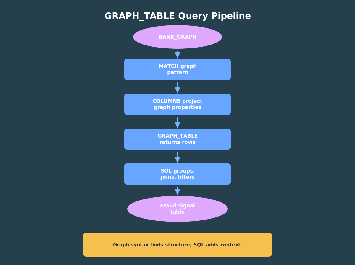
GRAPH_TABLE is a SQL table expression. You give it a graph and a pattern to match, and it returns rows. That last part matters. Once the graph match becomes rows, you can use the rest of SQL: joins, filters, grouping, ordering, and common table expressions.

Article 2 created BANK_GRAPH. This article uses that graph to show why pattern matching is worth learning: it lets you express fraud questions about hubs, chains, and cycles more directly than equivalent join-heavy SQL, while still returning rows that join to customer risk data.

In this article, we will query four fraud-style patterns:

inbound hubs;
two-hop transfer chains;
transfer cycles;
graph results joined to customer risk data.

Before you start, you’ll need to run the setup code from Article 2. I have copied that here so you can do it all in the one place. Make sure you use the “Run Script” button so it runs all of the statements, not just the first one.

Then run this code:

Ok, now you have everything that we did in the previous two articles back in place!

Now here’s the code for this example:

If you prefer to run everything in ADB-S, copy those three scripts into the same schema and run them in order. SQLcl and SQL*Plus users can run the files directly from the command line.

Before looking at each query, notice the repeated shape. The graph pattern lives inside GRAPH_TABLE, and the rest of the statement is ordinary SQL. That split is the core habit to learn: use graph syntax to find connected structures, then use SQL to summarize and enrich the results.

Pattern 1: Inbound Hubs

A simple first fraud question is: which accounts receive the most transfers?

In graph terms, we are looking for transfer edges that point into the same destination account.

			
SELECT gt.account_id,
       ba.account_name,
       COUNT(*) AS inbound_transfers,
       SUM(gt.amount) AS inbound_amount
FROM GRAPH_TABLE(
  bank_graph
  MATCH (src IS account) -[t IS transfer]-> (dst IS account)
  COLUMNS (
    dst.account_id AS account_id,
    t.amount AS amount
  )
) gt
JOIN bank_accounts ba
  ON ba.account_id = gt.account_id
GROUP BY gt.account_id, ba.account_name
ORDER BY inbound_transfers DESC, inbound_amount DESC;

		

The pattern is the important line:

MATCH (src IS account) -[t IS transfer]-> (dst IS account)

Read it from left to right: find an account vertex, follow a directed transfer edge, and land on another account vertex.

The COLUMNS clause chooses which graph properties become SQL columns. Here we project the destination account id and transfer amount. The outer SQL query groups those rows to find inbound hubs.

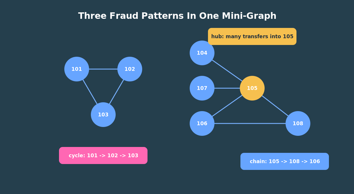
For the demo data, account 105 should stand out because several transfers point into it. That result is not automatically suspicious, but it is a useful triage signal. In a real system, you would combine it with time windows, amount thresholds, customer risk, and historical behavior.

Pattern 2: Accounts In The Middle

A second question is more interesting: which accounts sit in the middle of two-hop money movement?

That pattern looks like this:

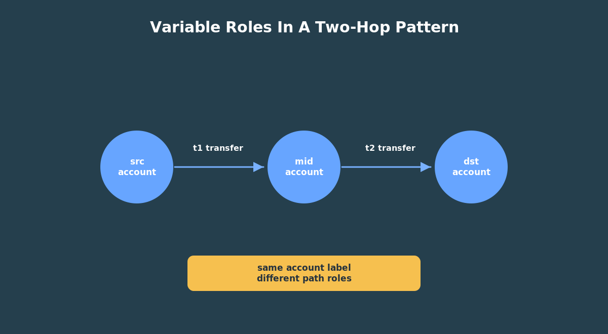
(source account)-[transfer]->(middle account)-[transfer]->(destination account)

The SQL graph query is direct:

			
SELECT gt.middle_account_id,
       ba.account_name,
       COUNT(*) AS times_in_middle,
       SUM(gt.first_amount + gt.second_amount) AS total_chain_amount
FROM GRAPH_TABLE(
  bank_graph
  MATCH (src IS account) -[t1 IS transfer]-> (mid IS account) -[t2 IS transfer]-> (dst IS account)
  COLUMNS (
    mid.account_id AS middle_account_id,
    t1.amount AS first_amount,
    t2.amount AS second_amount
  )
) gt
JOIN bank_accounts ba
  ON ba.account_id = gt.middle_account_id
GROUP BY gt.middle_account_id, ba.account_name
ORDER BY times_in_middle DESC, total_chain_amount DESC;

		

This is where graph syntax starts to feel natural. You are not mentally building a chain of self-joins. You are drawing the relationship pattern and asking Oracle to return the matches.

This query also shows why aliases matter. src, mid, and dst are not table names. They are pattern variables. The same account label appears three times, but each occurrence has a different role in the path. Good variable names make graph patterns much easier to explain on screen.

Pattern 3: Transfer Cycles

Fraud investigations often care about circular movement. Money leaves one account, moves through other accounts, and eventually returns.

The demo data has a simple cycle:

101 -> 102 -> 103 -> 101

In graph terms, we want to start at an account and return to the same account after a few transfer hops.

			
SELECT gt.account_id,
       ba.account_name,
       COUNT(*) AS cycle_count
FROM GRAPH_TABLE(
  bank_graph
  MATCH (a IS account) -[IS transfer]->{3,5} (a)
  COLUMNS (
    a.account_id AS account_id
  )
) gt
JOIN bank_accounts ba
  ON ba.account_id = gt.account_id
GROUP BY gt.account_id, ba.account_name
ORDER BY cycle_count DESC, gt.account_id;

		

The {3,5} quantifier is the part to notice. It asks for paths of three to five repetitions of the transfer step. The final (a) says the path must return to the same starting account.

The graph query expresses the business question almost exactly: “find accounts that can reach themselves through three to five transfers.”

Pattern 4: Join Graph Results To Customer Risk

Graph results are useful by themselves, but they become much more useful when you join them to business context.

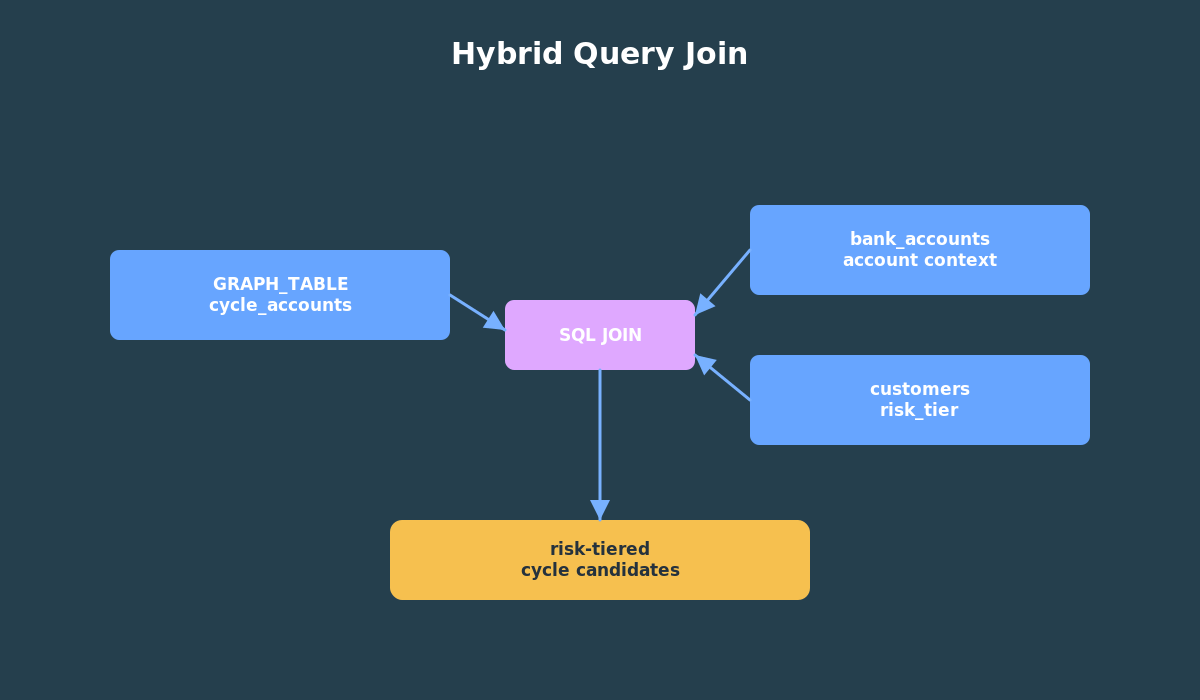
For example, a cycle involving a low-risk account may be less urgent than a cycle involving a high-risk customer. Because GRAPH_TABLE returns rows, we can join cycle results to bank_accounts and customers.

			
WITH cycle_accounts AS (
  SELECT account_id, COUNT(*) AS cycle_count
  FROM GRAPH_TABLE(
    bank_graph
    MATCH (a IS account) -[IS transfer]->{3,5} (a)
    COLUMNS (
      a.account_id AS account_id
    )
  )
  GROUP BY account_id
)
SELECT c.customer_id,
       c.full_name,
       c.risk_tier,
       ba.account_id,
       ba.account_name,
       ca.cycle_count
FROM cycle_accounts ca
JOIN bank_accounts ba
  ON ba.account_id = ca.account_id
JOIN customers c
  ON c.customer_id = ba.customer_id
WHERE c.risk_tier IN ('MEDIUM', 'HIGH')
ORDER BY ca.cycle_count DESC, c.risk_tier DESC, ba.account_id;

		

This is one of the strongest reasons to learn graph inside Oracle Database. You do not have to choose between graph analysis and relational context. You can combine them in one SQL workflow.

That is the practical payoff of this article. GRAPH_TABLE does not trap you in a graph-only world. It gives you a row source. Once you have rows, the rest of your SQL skills still apply.

What To Watch For

Graph syntax makes connected questions easier to read, but it does not remove the need for careful modeling.

Use stable keys for vertices and edges. Expose only the properties readers or applications need. Keep labels clear. Make edge direction explicit. If your business question treats relationships as undirected, say that clearly and choose the right query or algorithm path.

Next Step

Pattern matching answers many practical questions. But sometimes you want a computed signal: an importance score, a connected group id, or a weighted distance from a seed account.

That is where in-database graph algorithms come in. The next article uses DBMS_OGA in ADB-S, because the tested FreeSQL environment does not expose the algorithm packages. It then moves the same graph into Graph Studio for visualization.

That is also where edge weights become concrete. In the next article, the amount property on a transfer edge becomes the weight for a path example, instead of remaining an abstract graph term.

Try The Demo

The hands-on part of this article is the pattern-query script. It uses the BANK_GRAPH you created in Article 2 and runs the four query families you just learned:

inbound hubs;
two-hop transfer chains;
transfer cycles;
graph results joined to customer risk.

Use the embedded FreeSQL runner near the top of the article for the quick path. If you prefer ADB-S, run the same script in the schema where BANK_GRAPH already exists.

When the script finishes, spend a minute with the output instead of rushing ahead. Look for account 105 in the inbound hub result, the middle-account counts in the two-hop result, and the medium/high-risk customers in the hybrid query. Those outputs are the bridge between graph pattern matching and the algorithm examples in the next article.