The first article introduced the graph idea: vertices are things, edges are relationships, and properties describe both.

Now we will build one.

The easiest way to learn SQL property graphs in Oracle AI Database 26ai is to start with ordinary tables. That keeps the graph concrete. You can see the rows first, then see how the graph definition gives those rows a connected shape.

The point of this article is simple: you can create a queryable fraud graph on top of existing Oracle tables in one SQL statement, without duplicating the underlying data. By the end, you will have run the seed SQL, created BANK_GRAPH, and inspected the metadata Oracle stores for the graph.

In this article, we will create a small bank dataset and define a graph named BANK_GRAPH.

Start With Tables, Not Theory

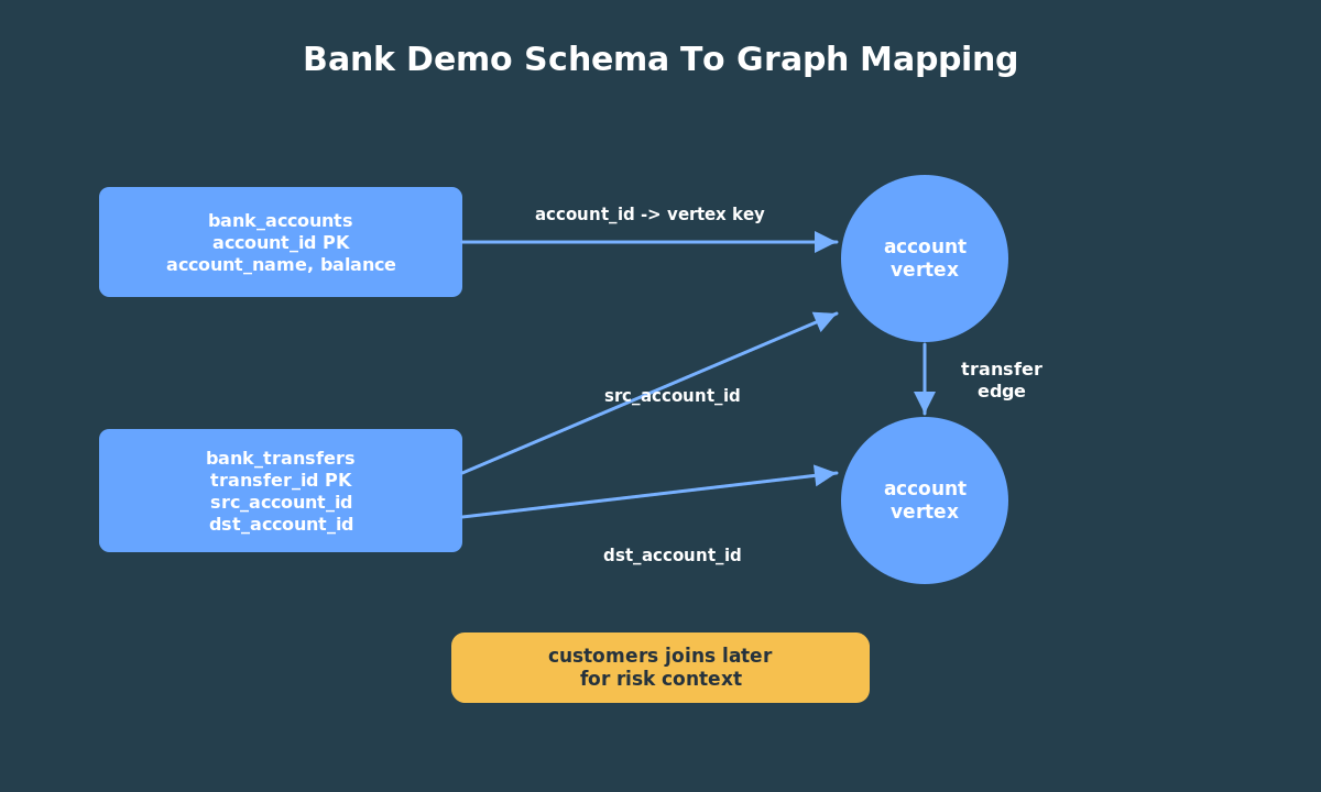
Our fraud example has three tables:

• customers, which stores customer names and risk tiers;
• bank_accounts, which stores account records;
• bank_transfers, which stores money movement from one account to another.

The transfer table is the key. Every transfer has a source account and a destination account. That is already an edge hiding in relational form.

This is why the example works well for a first graph. We do not have to invent a relationship. The relationship already exists in the schema; the graph definition just makes it explicit and queryable as a path.

The demo seed data includes a few useful patterns:

• a 3-hop cycle: 101 -> 102 -> 103 -> 101;
• a fan-in pattern where several accounts send money to account 105;
• a two-hop chain where account 105 sends to 108, and 108 sends to 106;
• customer risk tiers that we can join back to graph results later.

First, create the three tables, load the small dataset, and print row counts. Make sure you flip the switch to enable read/write so you can create new objects! If you do not, you will get an “insufficient privileges” error.

If you prefer to work in your own Autonomous Database Serverless instance, copy the same script into SQL Worksheet and run it there. SQLcl and SQL*Plus users can run the file directly from the command line.

When it finishes, you should see row counts for customers, accounts, and transfers.

This first tutorial deliberately avoids Object Storage and bulk-loading APIs. Those matter for production data, but they add noise to a beginner lesson whose real goal is graph modeling.

Define The Graph Vocabulary

The graph definition answers four questions:

• Which table contains vertices?
• Which table contains edges?
• Which columns identify each vertex and edge?
• Which properties should graph queries expose?

For this demo, bank_accounts becomes the vertex table and bank_transfers becomes the edge table.

Here is the essential graph definition:

CREATE OR REPLACE PROPERTY GRAPH bank_graph
  VERTEX TABLES (
    bank_accounts KEY (account_id)
      LABEL account
      PROPERTIES (account_id, customer_id, account_name, balance)
  )
  EDGE TABLES (
    bank_transfers KEY (transfer_id)
      SOURCE KEY (src_account_id) REFERENCES bank_accounts (account_id)
      DESTINATION KEY (dst_account_id) REFERENCES bank_accounts (account_id)
      LABEL transfer
      PROPERTIES (transfer_id, amount, transfer_ts, channel, note)
);

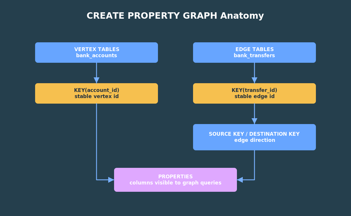
The VERTEX TABLES clause says that rows in bank_accounts are account vertices. The KEY clause says account_id uniquely identifies each vertex.

The EDGE TABLES clause says that rows in bank_transfers are transfer edges. The SOURCE KEY and DESTINATION KEY clauses make the edge direction explicit.

That direction matters. A transfer from account 101 to account 102 is not the same as a transfer from 102 to 101.

The PROPERTIES clauses are equally important. They decide which table columns are visible to graph queries. If you leave a column out, it remains available to ordinary SQL, but it will not be projected as a graph property in the graph pattern. For a teaching demo, keep the exposed properties small and obvious.

Next, create BANK_GRAPH and run the metadata checks shown below.

If you are using ADB-S instead, copy the code into the same schema where you ran the seed script.

Inspect The Graph

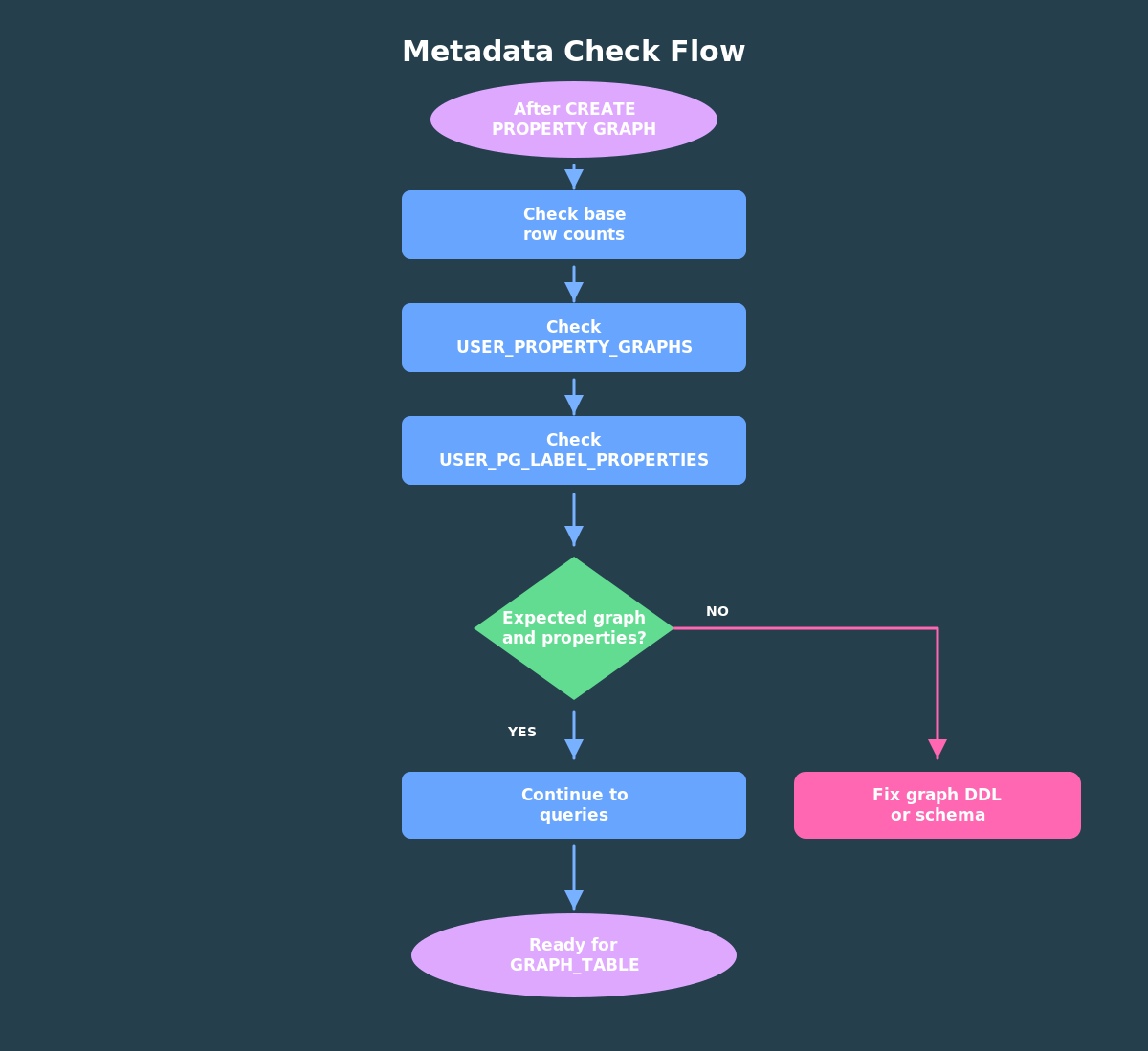
After the graph is created, inspect the database metadata.

The first check is simple:

SELECT graph_name
FROM user_property_graphs
WHERE graph_name = 'BANK_GRAPH';

That confirms that Oracle Database knows about the graph object.

Next, inspect the graph elements:

SELECT graph_name, element_name, element_kind, object_name
FROM user_pg_elements
WHERE graph_name = 'BANK_GRAPH'
ORDER BY element_kind, element_name;

You should see the account vertex element and the transfer edge element.

Then inspect labels and properties. This is useful when you are teaching or debugging because it shows the vocabulary that graph queries can use.

SELECT graph_name, label_name, property_name
FROM user_pg_label_properties
WHERE graph_name = 'BANK_GRAPH'
ORDER BY label_name, property_name;

The output should include properties such as ACCOUNT_ID, ACCOUNT_NAME, BALANCE, AMOUNT, CHANNEL, and TRANSFER_TS.

This metadata check is more than a sanity test. If a later graph query cannot see amount or account_name, the metadata views tell you whether the graph definition exposed those properties in the first place.

What The Graph Does Not Do

Creating BANK_GRAPH does not change the purpose of the base tables. Applications can still use customers, bank_accounts, and bank_transfers as ordinary relational tables.

The graph also does not decide what is fraudulent. It gives you a way to ask connected-data questions. In later articles, those questions become signals: cycles, hub accounts, accounts in the middle of transfer chains, PageRank scores, and connected groups. A real fraud workflow would combine those signals with business rules, investigation history, KYC data, device information, and human review.

The graph helps you see connection patterns. It does not magically replace risk modeling.

A Quick Check Before Moving On

Before you continue, make sure three things are true.

First, the base tables have rows. Second, USER_PROPERTY_GRAPHS shows BANK_GRAPH. Third, USER_PG_LABEL_PROPERTIES shows the properties you expect to query later, especially ACCOUNT_ID, ACCOUNT_NAME, AMOUNT, CHANNEL, and TRANSFER_TS.

Those checks are small, but they save time. Most beginner graph-query mistakes come from one of two places: the graph object was not created in the schema you are querying, or the property you want was not exposed in the graph definition.

If those checks pass, we can focus on patterns instead of setup. That is exactly where graph starts to feel different from ordinary table queries in practice.

Why This Matters

The graph is now ready, but the original data has not stopped being relational data.

That is the point. You can still query customers, bank_accounts, and bank_transfers with ordinary SQL. The graph adds a new query surface for connected patterns.

In the next article, we will use GRAPH_TABLE to ask questions like:

• Which accounts receive money from many sources?
• Which accounts sit in the middle of transfer chains?
• Which accounts are part of transfer cycles?
• Which suspicious graph results belong to high-risk customers?

Those questions are where the graph model starts to pay off.

Next step: move to Article 3, where the graph stops being metadata and starts answering fraud questions.

Try The Demo

This article had two runnable moments that you already saw above!

First, load the small bank dataset. That gives you ordinary relational tables with customers, accounts, and transfers. Second, create BANK_GRAPH over those tables and inspect the graph metadata.

Use the embedded FreeSQL runners above if you want the fastest path. Step 1 loads the data; Step 2 creates and checks the graph. If you prefer to use your own ADB-S instance, copy the same SQL into SQL Worksheet and run the scripts in the same order.

When both steps finish, you should have a graph named BANK_GRAPH in your schema. Keep it there for the next article. We will use that same graph to query hubs, two-hop chains, cycles, and customer-risk joins.