
GRAPH_TABLE is the right first tool because it demonstrates the core idea: match a graph pattern and return rows.
But graph work often goes one step further. You may want to rank important accounts, find connected groups, trace weighted paths, or visualize the network so a human can inspect it.
Article 3 used GRAPH_TABLE to find hubs, chains, cycles, and customer-risk joins. This article adds computed graph signals and visual exploration. You do not need a separate graph database after pattern matching; in-database algorithms and Graph Studio are the natural next step once you understand the graph.
Oracle gives you two practical next steps after basic pattern matching:
- in-database graph algorithms with
DBMS_OGA; - visual and notebook workflows in Graph Studio, backed by PGX for in-memory analytics.
Start With In-Database Algorithms
DBMS_OGA exposes graph algorithm functions that you can call from SQL. The function returns a temporary graph with computed properties, and GRAPH_TABLE reads those computed properties back as rows.
The syntax can look unusual at first, but the workflow is simple:
- call the algorithm on
BANK_GRAPH; - write the algorithm output to a vertex property;
- query that output property with
GRAPH_TABLE; - join the result to your relational tables.
Run the examples in this article in Autonomous Database Serverless on OCI if you want the algorithm examples to execute. At the time of writing, FreeSQL does not expose DBMS_OGA / DBMS_GAF, so the algorithm examples in this article will not work there.
If you are using ADB-S, run the setup from earlier articles first. Then check whether your database exposes the graph algorithm packages:
SELECT owner, object_name, object_type, statusFROM all_objectsWHERE object_name IN ('DBMS_OGA', 'DBMS_GAF')ORDER BY owner, object_name, object_type;
If that query does not show both packages, skip the DBMS_OGA examples in this article and move to the Graph Studio section.
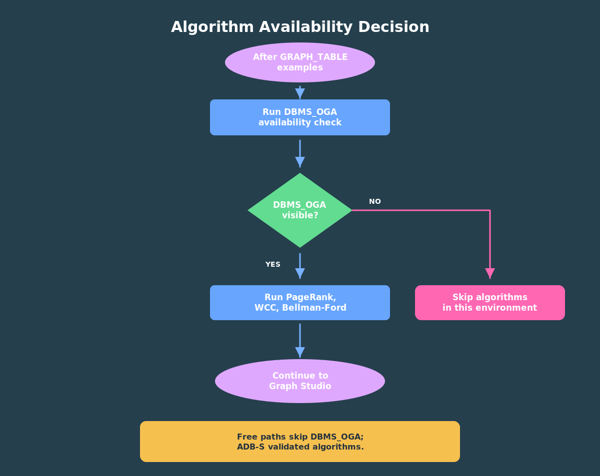
The algorithm path depends on DBMS_OGA and DBMS_GAF. If those packages are not visible in your environment, keep using the earlier SQL property graph and GRAPH_TABLE examples, then move to the Graph Studio section.
If DBMS_OGA is visible, run demo/04_bank_graph_algorithms.sql. (The code is at end of this article). The script checks package visibility first, skips cleanly where the packages are absent, and uses the current schema when it builds the Bellman-Ford seed vertex JSON.
Treat these algorithm outputs as features, not verdicts. A PageRank score, component id, or path distance can help you prioritize work, but it should not be presented as proof of fraud. That distinction keeps the article technically useful without overstating what graph analytics can decide on its own.
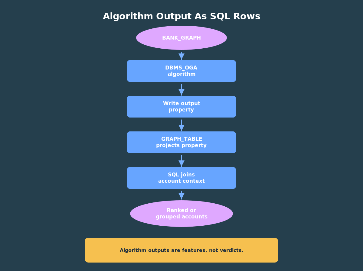
The useful part is not just that the algorithm runs. It is that the computed graph output can come back through GRAPH_TABLE, become SQL rows, and join to the same relational context you already use.
PageRank: Which Accounts Are Structurally Important?
PageRank is a useful first centrality measure because it gives every vertex an importance score based on the graph structure.
In a bank-transfer graph, PageRank is not a fraud model. It is a signal. An account with high graph importance may deserve attention when combined with other context such as transfer amount, customer risk, device history, or known investigation seeds.
SELECT gt.account_id, ba.account_name, gt.pagerank_scoreFROM GRAPH_TABLE( DBMS_OGA.PAGERANK( bank_graph, PROPERTY(VERTEX OUTPUT pagerank_score), 20, 0.0001, 0.85, TRUE ) MATCH (a IS account) COLUMNS ( a.account_id AS account_id, a.pagerank_score AS pagerank_score )) gtJOIN bank_accounts ba ON ba.account_id = gt.account_idORDER BY gt.pagerank_score DESC;
Notice the same pattern from earlier articles. Even though an algorithm ran first, the output becomes SQL rows. That makes the score easy to sort, filter, join, or save.
You can also join the result back to customer or account data. For example, sort by PageRank and then show each account’s customer risk tier. The algorithm provides graph structure; SQL adds business context.
Weakly Connected Components: Which Accounts Belong Together?
Connected components find groups of vertices connected by edges. Weakly connected components treat directed edges as connected regardless of direction.
In a fraud investigation workflow, WCC is useful because it gives you a compact way to describe account clusters.
SELECT gt.component_id, COUNT(*) AS account_count, LISTAGG(ba.account_name, ', ') WITHIN GROUP (ORDER BY ba.account_id) AS accountsFROM GRAPH_TABLE( DBMS_OGA.WCC( bank_graph, PROPERTY(VERTEX OUTPUT component_id) ) MATCH (a IS account) COLUMNS ( a.account_id AS account_id, a.component_id AS component_id )) gtJOIN bank_accounts ba ON ba.account_id = gt.account_idGROUP BY gt.component_idORDER BY account_count DESC, gt.component_id;
On a small graph, this may return one large component. That is fine. The useful pattern is the method: compute a graph-level grouping, then summarize it with SQL.
On a larger graph, connected components can help split an investigation into smaller clusters. They can also help you find isolated groups of accounts that do not interact with the rest of the network.
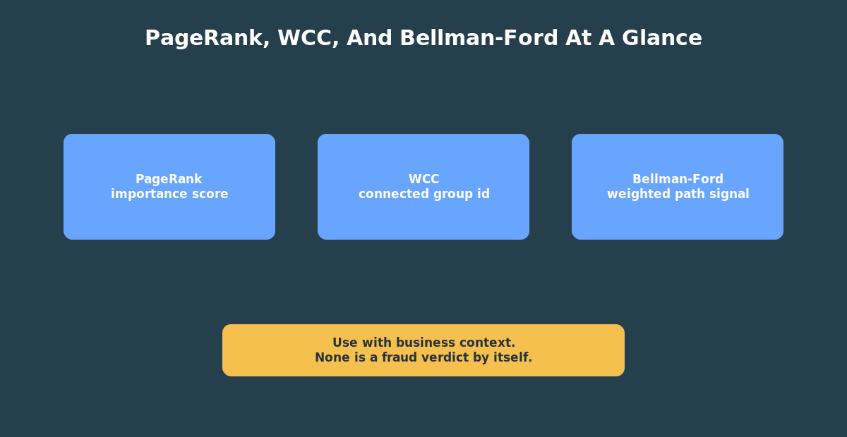
PageRank, Weakly Connected Components, and Bellman-Ford produce different kinds of graph features. Treat them as investigation inputs, not final decisions.
Bellman-Ford: Weighted Path Exposure
Bellman-Ford is a shortest-path algorithm. In a road network, the edge weight might be distance. In a transfer graph, the edge weight might be amount.
In this demo, a minimum cumulative transfer amount is not automatically a risk score. It is a path-based measure that may help investigation when paired with business rules.
The Bellman-Ford example starts from account 101 and uses transfer amount as the edge weight.
The seed vertex is account 101. The edge input property is amount, so the algorithm treats transfer amount as the path weight. The output property is minimum_transfer_exposure, which is then projected by GRAPH_TABLE and joined to bank_accounts.
This output is a weighted path signal from one starting account. In an investigation workflow, it could help you understand which accounts are reachable from a seed account under this weighting rule.
Move Into Graph Studio
SQL is enough to create and query the graph, but visualization helps beginners see what they built.
Graph Studio gives you a managed place to create, query, analyze, and visualize graphs in Autonomous AI Database. In this series, it is most useful for three things:
- show
BANK_GRAPHas a real graph object; - visualize a small subgraph around account
101; - run one notebook or query-panel example that mirrors the SQL article.
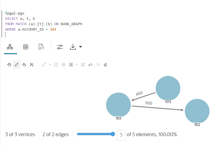
In Graph Studio, open the graph list, select BANK_GRAPH, and start with a small preview rather than the whole graph. Filter around account 101 or the 3-hop cycle so the visual reinforces the pattern queries instead of turning into a dense tangle.
If you use a notebook, run the same one-hop query from account 101 that you used in SQL. That helps connect the visual result back to the query:
SELECT *FROM GRAPH_TABLE( bank_graph MATCH (src IS account) -[t IS transfer]-> (dst IS account) WHERE src.account_id = 101 COLUMNS ( src.account_name AS source_account, t.amount AS amount, t.channel AS channel, dst.account_name AS destination_account ))ORDER BY amount DESC;
Where PGX Fits
PGX is Oracle’s in-memory graph analytics layer. It matters when you need richer algorithms, interactive analysis, notebook workflows, or high-performance graph analytics beyond the first SQL examples.
The practical path is incremental: start in SQL, add in-database algorithm signals when the packages are available, and move into Graph Studio or PGX when visualization or deeper analytics becomes useful.
That sequence keeps the mental model clean:
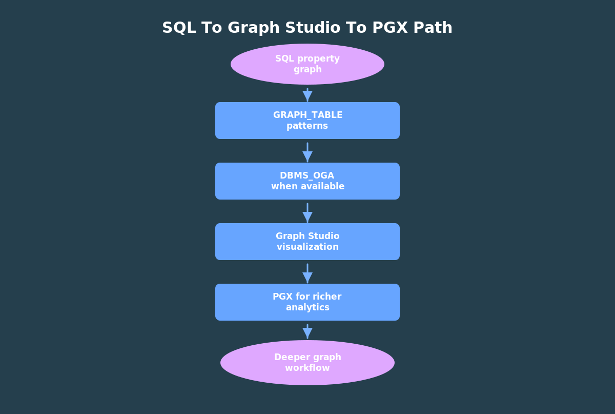
- SQL property graph: define the graph over database objects.
GRAPH_TABLE: match graph patterns and return rows.DBMS_OGA: compute basic in-database graph signals.- Graph Studio and PGX: visualize and analyze with a richer graph environment.
Where To Go Next
You now know how to recognize a graph-shaped problem, define a SQL property graph over relational tables, query connected patterns with SQL, join graph results to business context, and choose when to move into algorithms or visualization.
That is enough to start using graph features in real Oracle database work.
Try The Demo
This article has two demo paths.
For the algorithm path, use your own ADB-S instance. Run the setup steps below, then run the availability check and algorithm script. The script computes PageRank, Weakly Connected Components, and Bellman-Ford outputs, then returns the results as SQL rows.
For the FreeSQL path, stop before the algorithm script. FreeSQL is still useful for the table, graph, and GRAPH_TABLE pattern examples, but FreeSQL does not expose DBMS_OGA / DBMS_GAF.
After the SQL algorithm step, open Graph Studio in the same ADB-S environment and visualize a small part of BANK_GRAPH. Start with a filtered view around account 101 or the seeded transfer cycle. The goal is not to draw every relationship at once; it is to connect the SQL results back to a graph a person can inspect.
Here’s the code referenced above, which you can copy and paste into your environment. Please note that you need to run the set up steps 1 and 2 first, then step 4 – all are included below. If you followed the previous articles in this series, steps 1 and 2 are exactly the same code you ran in those articles. The code below contains comments that explains what it is doing.
-- Oracle AI Database 26ai graph demo-- Step 1: create a tiny bank-fraud dataset.---- Run this as a schema user that can create tables.-- Start by removing objects from a previous run. The graph depends on the-- tables, so it must be dropped before the tables can be recreated.BEGIN EXECUTE IMMEDIATE 'DROP PROPERTY GRAPH bank_graph';EXCEPTION WHEN OTHERS THEN -- Ignore cleanup errors so the script can be rerun from a fresh schema or -- after dependencies have already been removed. NULL;END;/-- Drop the edge table before the vertex tables because it has foreign keys to-- bank_accounts. ORA-00942 means the table did not exist, which is safe here.BEGIN EXECUTE IMMEDIATE 'DROP TABLE bank_transfers PURGE';EXCEPTION WHEN OTHERS THEN IF SQLCODE != -942 THEN RAISE; END IF;END;/-- Drop bank_accounts after bank_transfers because transfers reference accounts.BEGIN EXECUTE IMMEDIATE 'DROP TABLE bank_accounts PURGE';EXCEPTION WHEN OTHERS THEN IF SQLCODE != -942 THEN RAISE; END IF;END;/-- Drop the parent customer table last because bank_accounts references it.BEGIN EXECUTE IMMEDIATE 'DROP TABLE customers PURGE';EXCEPTION WHEN OTHERS THEN IF SQLCODE != -942 THEN RAISE; END IF;END;/-- Customers are the business owners of accounts. The risk_tier column gives us-- a simple relational attribute to join back to graph query results later.CREATE TABLE customers ( customer_id NUMBER NOT NULL, full_name VARCHAR2(100) NOT NULL, risk_tier VARCHAR2(20) NOT NULL, CONSTRAINT customers_pk PRIMARY KEY (customer_id), CONSTRAINT customers_risk_chk CHECK (risk_tier IN ('LOW', 'MEDIUM', 'HIGH')));-- Accounts will become graph vertices in 02_bank_graph.sql. Each account is-- still normal relational data, including a foreign key back to customers.CREATE TABLE bank_accounts ( account_id NUMBER NOT NULL, customer_id NUMBER NOT NULL, account_name VARCHAR2(100) NOT NULL, balance NUMBER(12,2) NOT NULL, CONSTRAINT bank_accounts_pk PRIMARY KEY (account_id), CONSTRAINT bank_accounts_customer_fk FOREIGN KEY (customer_id) REFERENCES customers (customer_id));-- Transfers will become directed graph edges. The source and destination-- account IDs define the arrow direction for graph pattern matching.CREATE TABLE bank_transfers ( transfer_id NUMBER NOT NULL, src_account_id NUMBER NOT NULL, dst_account_id NUMBER NOT NULL, amount NUMBER(12,2) NOT NULL, transfer_ts TIMESTAMP NOT NULL, channel VARCHAR2(30) NOT NULL, note VARCHAR2(200), CONSTRAINT bank_transfers_pk PRIMARY KEY (transfer_id), CONSTRAINT bank_transfers_src_fk FOREIGN KEY (src_account_id) REFERENCES bank_accounts (account_id), CONSTRAINT bank_transfers_dst_fk FOREIGN KEY (dst_account_id) REFERENCES bank_accounts (account_id), CONSTRAINT bank_transfers_amount_chk CHECK (amount >= 0));-- Load a small mix of low-, medium-, and high-risk customers so later examples-- can combine graph patterns with ordinary relational filters.INSERT INTO customers (customer_id, full_name, risk_tier) VALUES (1, 'Avery Chen', 'LOW'), (2, 'Blake Rao', 'MEDIUM'), (3, 'Casey Morgan', 'HIGH'), (4, 'Drew Singh', 'LOW'), (5, 'Emery Stone', 'HIGH'), (6, 'Finley Brooks', 'MEDIUM');-- Give some customers multiple accounts. This makes the graph slightly more-- realistic without requiring a large dataset.INSERT INTO bank_accounts (account_id, customer_id, account_name, balance) VALUES (101, 1, 'Avery checking', 8400.00), (102, 2, 'Blake checking', 1250.00), (103, 3, 'Casey operating', 620.00), (104, 4, 'Drew savings', 15000.00), (105, 5, 'Emery wallet', 210.00), (106, 6, 'Finley checking', 3700.00), (107, 3, 'Casey reserve', 480.00), (108, 5, 'Emery reserve', 305.00);-- A 3-hop cycle: 101 -> 102 -> 103 -> 101.-- This gives the GRAPH_TABLE examples a compact round-trip pattern to find.INSERT INTO bank_transfers ( transfer_id, src_account_id, dst_account_id, amount, transfer_ts, channel, note) VALUES (1001, 101, 102, 500.00, TIMESTAMP '2026-05-01 09:00:00', 'ACH', 'invoice payment'), (1002, 102, 103, 475.00, TIMESTAMP '2026-05-01 09:14:00', 'ACH', 'same-day transfer'), (1003, 103, 101, 450.00, TIMESTAMP '2026-05-01 09:37:00', 'WIRE', 'round trip');-- A fan-in pattern around account 105.-- Multiple incoming transfers make account 105 stand out as an inbound hub.INSERT INTO bank_transfers ( transfer_id, src_account_id, dst_account_id, amount, transfer_ts, channel, note) VALUES (1004, 104, 105, 850.00, TIMESTAMP '2026-05-02 10:00:00', 'WIRE', 'vendor settlement'), (1005, 106, 105, 920.00, TIMESTAMP '2026-05-02 10:03:00', 'WIRE', 'vendor settlement'), (1006, 107, 105, 760.00, TIMESTAMP '2026-05-02 10:06:00', 'WIRE', 'vendor settlement');-- A second chain with a high-risk customer in the middle.-- These rows support the two-hop path examples and the relational risk join.INSERT INTO bank_transfers ( transfer_id, src_account_id, dst_account_id, amount, transfer_ts, channel, note) VALUES (1007, 105, 108, 700.00, TIMESTAMP '2026-05-02 11:10:00', 'ACH', 'split transfer'), (1008, 108, 106, 690.00, TIMESTAMP '2026-05-02 11:30:00', 'ACH', 'split transfer'), (1009, 106, 107, 300.00, TIMESTAMP '2026-05-03 13:00:00', 'CARD', 'refund'), (1010, 107, 102, 290.00, TIMESTAMP '2026-05-03 13:20:00', 'CARD', 'refund');-- Make the seed data visible to the following scripts.COMMIT;-- Quick smoke test: the expected row counts are 6 customers, 8 accounts, and-- 10 transfers.SELECT 'customers' AS table_name, COUNT(*) AS rows_loaded FROM customersUNION ALLSELECT 'bank_accounts', COUNT(*) FROM bank_accountsUNION ALLSELECT 'bank_transfers', COUNT(*) FROM bank_transfers;-- Oracle AI Database 26ai graph demo-- Step 2: create a SQL property graph over the bank tables.-- A SQL property graph is metadata over existing relational tables. This-- statement does not copy the rows from bank_accounts or bank_transfers; it-- describes how Oracle should treat those rows as graph vertices and edges.---- In this graph:-- - bank_accounts rows become account vertices, keyed by account_id.-- - bank_transfers rows become directed transfer edges, keyed by transfer_id.-- - SOURCE KEY and DESTINATION KEY define transfer direction.-- - PROPERTIES lists the columns that graph queries can project.CREATE OR REPLACE PROPERTY GRAPH bank_graph VERTEX TABLES ( bank_accounts KEY (account_id) LABEL account PROPERTIES (account_id, customer_id, account_name, balance) ) EDGE TABLES ( bank_transfers KEY (transfer_id) SOURCE KEY (src_account_id) REFERENCES bank_accounts (account_id) DESTINATION KEY (dst_account_id) REFERENCES bank_accounts (account_id) LABEL transfer PROPERTIES (transfer_id, amount, transfer_ts, channel, note) );-- Confirm that the graph object exists in the current schema.SELECT graph_nameFROM user_property_graphsWHERE graph_name = 'BANK_GRAPH';-- Inspect the graph elements. You should see one vertex element backed by-- BANK_ACCOUNTS and one edge element backed by BANK_TRANSFERS.SELECT graph_name, element_name, element_kind, object_nameFROM user_pg_elementsWHERE graph_name = 'BANK_GRAPH'ORDER BY element_kind, element_name;-- Inspect graph labels. Labels are the names used in MATCH patterns such as-- (a IS account) and -[t IS transfer]->.SELECT graph_name, label_nameFROM user_pg_labelsWHERE graph_name = 'BANK_GRAPH'ORDER BY label_name;-- Inspect the properties available for each label. If a column is not listed-- here, a GRAPH_TABLE query cannot project it as a graph property.SELECT graph_name, label_name, property_nameFROM user_pg_label_propertiesWHERE graph_name = 'BANK_GRAPH'ORDER BY label_name, property_name;-- Capture the canonical graph DDL for source control or an article appendix.-- This is also a useful way to compare what you wrote with what Oracle stores.SELECT DBMS_METADATA.GET_DDL('PROPERTY_GRAPH', 'BANK_GRAPH') AS graph_ddlFROM dual;-- Oracle AI Database 26ai graph demo-- Step 4: run in-database graph algorithms with DBMS_OGA.---- IMPORTANT:-- Run after 01_bank_schema_and_seed.sql and 02_bank_graph.sql.-- This script requires DBMS_OGA and DBMS_GAF to be installed/visible.-- The tested FreeSQL, ADB Free, and Oracle Database Free environments support-- SQL property graphs and GRAPH_TABLE, but do not expose DBMS_OGA / DBMS_GAF.---- The algorithm SQL is deliberately executed dynamically after the package-- check. In environments where DBMS_OGA is not installed, static SQL can fail-- during GRAPH_TABLE parsing with ORA-02000: missing MATCH keyword.-- DBMS_OUTPUT prints the availability check and section headings. SQL Developer-- Web and SQLcl can also display the result sets returned by DBMS_SQL.SET SERVEROUTPUT ON SIZE UNLIMITEDDECLARE -- The package count is used as a gate so FreeSQL and other environments -- without DBMS_OGA / DBMS_GAF exit cleanly instead of failing mid-script. l_package_count NUMBER; -- Bellman-Ford needs a JSON seed vertex that includes the graph owner. Using -- the current schema keeps the script portable across demo users. l_graph_owner VARCHAR2(128) := SYS_CONTEXT('USERENV', 'CURRENT_SCHEMA'); -- Each algorithm query is stored as text and opened dynamically only after -- the package check succeeds. l_sql VARCHAR2(32767); -- Run one algorithm query, label the output, and return the cursor to the SQL -- client as a result set. If one algorithm fails, the message explains which -- section failed without hiding the earlier successful sections. PROCEDURE run_result(p_title VARCHAR2, p_sql VARCHAR2) IS l_cursor SYS_REFCURSOR; BEGIN DBMS_OUTPUT.PUT_LINE(CHR(10) || '=== ' || p_title || ' ==='); OPEN l_cursor FOR p_sql; DBMS_SQL.RETURN_RESULT(l_cursor); EXCEPTION WHEN OTHERS THEN DBMS_OUTPUT.PUT_LINE('FAILED: ' || p_title); DBMS_OUTPUT.PUT_LINE(SQLERRM); END;BEGIN -- Confirm both graph algorithm packages are visible before referencing them -- inside GRAPH_TABLE. They may be unavailable in FreeSQL and Free images. SELECT COUNT(DISTINCT object_name) INTO l_package_count FROM all_objects WHERE object_name IN ('DBMS_OGA', 'DBMS_GAF') AND object_type IN ('PACKAGE', 'SYNONYM'); IF l_package_count < 2 THEN DBMS_OUTPUT.PUT_LINE('DBMS_OGA / DBMS_GAF are not both visible in this environment.'); DBMS_OUTPUT.PUT_LINE('Skip the in-database algorithm examples.'); RETURN; END IF; DBMS_OUTPUT.PUT_LINE('DBMS_OGA / DBMS_GAF are visible.'); DBMS_OUTPUT.PUT_LINE('Using graph owner for Bellman-Ford seed JSON: ' || l_graph_owner); -- PageRank scores each account by its graph importance based on transfer -- relationships. The algorithm writes pagerank_score as a temporary vertex -- property, and GRAPH_TABLE projects it back into SQL rows. run_result( 'PageRank', q'[ SELECT gt.account_id, ba.account_name, gt.pagerank_score FROM GRAPH_TABLE( DBMS_OGA.PAGERANK( bank_graph, PROPERTY(VERTEX OUTPUT pagerank_score), 20, 0.0001, 0.85, TRUE ) MATCH (a IS account) COLUMNS ( a.account_id AS account_id, a.pagerank_score AS pagerank_score ) ) gt JOIN bank_accounts ba ON ba.account_id = gt.account_id ORDER BY gt.pagerank_score DESC ]' ); -- Weakly connected components groups accounts that are connected when edge -- direction is ignored. In a fraud or risk workflow, components can reveal -- clusters that should be reviewed together. run_result( 'Weakly Connected Components', q'[ SELECT gt.component_id, COUNT(*) AS account_count, LISTAGG(ba.account_name, ', ') WITHIN GROUP (ORDER BY ba.account_id) AS accounts FROM GRAPH_TABLE( DBMS_OGA.WCC( bank_graph, PROPERTY(VERTEX OUTPUT component_id) ) MATCH (a IS account) COLUMNS ( a.account_id AS account_id, a.component_id AS component_id ) ) gt JOIN bank_accounts ba ON ba.account_id = gt.account_id GROUP BY gt.component_id ORDER BY account_count DESC, gt.component_id ]' ); -- Bellman-Ford computes weighted reachability from account 101 using transfer -- amount as the edge weight. The JSON value identifies the seed vertex in the -- graph, so the schema name is filled in at runtime below. l_sql := q'[ SELECT gt.account_id, ba.account_name, gt.minimum_transfer_exposure FROM GRAPH_TABLE( DBMS_OGA.BELLMAN_FORD( bank_graph, JSON('{"GRAPH_OWNER":"__GRAPH_OWNER__","GRAPH_NAME":"BANK_GRAPH","ELEM_TABLE":"BANK_ACCOUNTS","KEY_VALUE":{"ACCOUNT_ID":101}}'), PROPERTY(EDGE INPUT amount DEFAULT ON NULL 0), PROPERTY(VERTEX OUTPUT minimum_transfer_exposure) ) MATCH (a IS account) COLUMNS ( a.account_id AS account_id, a.minimum_transfer_exposure AS minimum_transfer_exposure ) ) gt JOIN bank_accounts ba ON ba.account_id = gt.account_id ORDER BY gt.minimum_transfer_exposure, gt.account_id ]'; -- Replace the placeholder after building the SQL string so the script works -- regardless of the schema name used for the demo. l_sql := REPLACE(l_sql, '__GRAPH_OWNER__', l_graph_owner); run_result('Bellman-Ford', l_sql);END;/

You must be logged in to post a comment.